-
1500 words • 8 min read • Abstract
AI Tools #4: Pi --- The Minimal Agent That Stays Out of the Way

Four tools. Read, Write, Edit, Bash.
That is the part of Pi that looks like a slogan, but after using it the point feels less like minimalism for its own sake and more like friction control. Pi is not trying to become the center of the development environment. It is a small agent loop that can read files, change files, run commands, and leave the rest of the system alone.
My setup makes that especially visible. I use
moshfrom my MacBook to connect to an Arch Linux server, because it survives network hiccups better than plainssh. On that server I log into an unprivileged user account and runtmux, which gives me multiple persistent PTYs. One tmux window runs Pi withgemma4on an RTX 3090 with 24 GB of VRAM. Another tmux window is just a shell prompt, or sometimes an Emacs shell.I use the same general pattern for other coding agents: Claude Code, Codex, Gemini, and opencode using the Z.ai dev plan with GLM-5. That makes Pi’s shape easier to compare. The machine, project, shell, and tmux workflow stay mostly constant. What changes is how much agent framework shows up before the model starts doing useful work.
That makes Pi a useful counterweight to the current agent-tooling habit of turning every workflow into a platform.
Resource Link Pi Mono Repo badlogic/pi-mono Armin’s Extensions mitsuhiko/agent-stuff Article Pi: The Minimal Agent Lucy short YouTube Comments Discord The Working Shape
My current Pi setup is not a cloud-agent command center. It is a local model, a default thinking level, and one package:
{
  "defaultModel": "gemma4",
  "defaultProvider": "ollama",
  "lastChangelogVersion": "0.74.0",
  "packages": [
    "npm:@ollama/pi-web-search"
  ],
  "defaultThinkingLevel": "medium"
}
That lives at:
~/.pi/agent/settings.jsonMotivation
The practical motivation is Lucy, my local AI cluster (short video). I want local LLMs to take on simpler development tasks without every small question or edit going out to a frontier model.
That does not mean pretending a local model is equivalent to Claude, Codex, Gemini, or GLM-5 on every task. It means finding the band of work where locality, cost, privacy, and iteration speed matter more than maximum model strength.
I have been using opencode for that local-agent lane, and Pi is another experiment in the same direction. The question is not just whether this agent can solve a task. It is whether this agent makes local-model development feel cheap enough and clear enough that I will use it repeatedly.
The longer-term plan is to fine-tune local models so they get better at my specific tasks over time. I want agents that can learn from their mistakes instead of merely forgetting them after the session ends.
This is the interesting version of Pi to me: not “look how many integrations this has,” but “look how little standing machinery needs to be loaded before the model can start doing useful work.” A local Ollama model is enough to keep the loop close. One web-search package is enough to give it a narrow escape hatch when local context is not enough. The rest is just the agent doing agent things against the current working directory.
Pi matters in that context because its loop is small enough to observe. If I want to turn agent experience into future training data, I need transcripts and actions that are easy to understand. A minimal agent loop is not just easier for me to debug today; it is cleaner raw material for tomorrow’s local learning pipeline.
Minimal Does Not Mean Weak
The core tool set is boring:
Tool Job Read Inspect files Write Create or replace files Edit Patch existing files Bash Run commands Those four operations cover a surprising amount of software work because most coding-agent work eventually becomes:
- inspect the repo,
- make a small change,
- run the command that proves or falsifies it,
- repeat.
That is not everything an agent might do. It is, however, the irreducible loop under a lot of the tooling we dress up with dashboards, plugin catalogs, project memories, task graphs, and elaborate orchestration.
The point is not that Pi uses a smaller context window. Pi can use whatever context window the selected model supports. The optimization is that Pi spends less of that window on the agent framework itself. More of the model’s available attention can go to the repo, the task, the transcript, and the command output that actually matter.
What Pi Gets Right
Pi’s strength is that it does not make the agent feel more magical than it is. The model can read, edit, and run commands. If the result is wrong, the failure is usually visible in the transcript or the filesystem.
That matters. Agent systems become hard to debug when too much behavior is hidden behind framework policy: tool routers, memory layers, implicit plans, autonomous retries, invisible summarizers. Those pieces can be useful, but they also make the system harder to reason about.
Pi’s small surface area gives it three practical advantages:
- Low ceremony: starting a session does not feel like launching infrastructure.
- Good failure shape: when it gets confused, the mistake is usually local.
- Efficient context use: the initial context is not crowded by unused capabilities.
- Easy composition: additional behavior can live outside the core loop.
That last point is the important one. Minimal systems survive contact with real work when they have an extension path. Pi’s philosophy is not “never add capabilities.” It is “do not pre-spend context on every capability someone might want someday.”
Local Models Change the Feel
Using Pi with Ollama changes the social contract of the tool. A local model is not always the smartest model in the room, but it is cheap to call, private by default, and always available when the machine is available.
That makes Pi useful for narrower work than I would hand to a frontier coding agent:
- asking it to inspect a small code path,
- generating a first-pass script,
- trying a quick refactor in a disposable branch,
- keeping a local search/edit/run loop warm while I think.
The settings file captures that stance.
gemma4viaollama, medium thinking, one web-search package. Enough help to be useful. Not enough machinery to become a second project.OpenClaw Is Context, Not the Headline
Pi is also part of a broader ecosystem. OpenClaw and related experiments build larger agent experiences on top of Pi-style pieces. That is worth mentioning because it proves the core can be embedded.
But for this post, OpenClaw is not the main point. The main point is that Pi itself is a clean reference design for a coding agent:
model + prompt + four tools + transcript + working directoryEverything else should have to justify itself.
The Slant After Using It
Before using Pi, the obvious story is “minimal agent has only four tools.” After using it, the better story is “minimal agents preserve mechanical sympathy by treating context as a working budget.”
You know what the agent can touch. You know what it can run. You know where configuration lives. You can look at the settings file and understand the operating posture in ten seconds:
- local model,
- local provider,
- medium reasoning effort,
- one explicit package.
That is a better baseline than most agent frameworks provide. A big model context window is still valuable. Pi’s advantage is that it does not fill that window with framework overhead before the problem has earned it.
Key Takeaways
-
The useful unit is the loop. Read, edit, run, observe is the center of coding-agent work.
-
Minimal cores age well. The less policy hidden in the core, the easier the system is to debug and extend.
-
Local models are a different workflow, not just a cheaper backend. Pi plus Ollama makes small, frequent agent use feel natural.
-
Context efficiency is an optimization, not a constraint. Pi can use the model’s full context when the task calls for it; it simply starts by spending fewer tokens on itself.
-
Extensions should orbit the core. Packages and integrations are useful, but they should not make the agent’s basic behavior mysterious.
Resources
Part 4 of the AI Tools series. View all parts | Next: Part 5 →
Comments or questions? SW Lab Discord or YouTube @SoftwareWrighter.

-
1699 words • 9 min read • Abstract
AI Tools #5: nono --- Sandboxing Pi Without Breaking the Loop

The promise of nono is simple: give an AI coding agent a real sandbox. Not a prompt-level warning. Not a policy reminder. A kernel-enforced boundary around what the process can read, write, delete, and contact.
That is exactly the kind of tool I want in the local-agent workflow from the Pi post. I am running agents on Lucy, my local AI cluster, through
mosh,tmux, unprivileged user accounts, and local models. If those agents are going to edit code and run commands, they need boundaries that do not depend on the model being obedient.But the path to a usable setup was not “install nono, run Pi, done.” It took a while to find a working combination of nono, Pi, Ollama, and an LLM that could do useful work without getting wedged.
Resource Link nono website nono.sh nono code lukehinds/nono nono docs docs.nono.sh Pi repo badlogic/pi-mono Lucy short YouTube Comments Discord The Goal
The goal was not theoretical sandbox purity. It was more practical:
- run Pi inside a constrained environment,
- let Pi use Ollama for a local model,
- allow enough filesystem access for useful development,
- prevent obvious damage or secret exposure,
- keep the loop small enough that failures are understandable.
That last point matters. Sandboxing an agent is not useful if the agent becomes too constrained to act, too confused to use its tools, or too wrapped in indirection to debug.
The Iteration Tax
The first cost was permission tuning.
nono is a capability boundary. That is the point. But agent work is full of little side effects: reading project files, writing scratch files, running commands, following symlinks, touching caches, calling helper binaries, connecting to a local model server, and sometimes discovering that the next thing it needs is outside the allowlist.
That creates a tuning loop:
run agent
watch it fail
inspect what was denied
adjust permissions
run again
Motivation
Recently I have had several experiences where a model — Claude, Gemma4 — unilaterally decided to remove a file or directory it did not understand.
That is astonishingly cavalier when the target was recently created and not yet tracked by git. There is no easy reflog recovery for a directory that never made it into the repository.
The contrast is strange: Claude constantly asks permission for simple, undoable things, but a model can still destroy local work if the command gets through. That starts to feel like security theater: prompts that throttle usage by causing more round trips, not structural safety.
I considered putting an rm wrapper earlier in PATH that just says no. But what stops a model from running /usr/bin/rm directly?
nono does.
Some failures are good. They prove the sandbox is doing its job. Other failures are friction: the agent cannot reach the local service it needs, cannot write where the tool expects, or gets confused by an environment that is almost but not quite normal.
This is where nono gets real. The hard part is not believing in sandboxing. The hard part is finding the permission set that is narrow enough to matter and wide enough to work.
When Models Talk Instead of Act
The second cost was model behavior.
I repeatedly hit a local-model failure mode where the model would describe what it was going to do instead of actually doing it. It would outline a plan, explain the next command, or narrate the intended edit, but not drive the tool loop forward, even after repeated cajoling to just do it.
That is a different problem from sandboxing. nono can enforce filesystem and process boundaries, but it cannot make a weak model become an effective coding agent. If the model does not reliably convert intent into tool calls, the safest sandbox in the world just protects a process that is not doing much.
That distinction is important:
Failure Layer Cannot read/write needed path Sandbox permissions Cannot reach Ollama Process/network/environment shape Describes the plan but does not act Model/tool-use behavior Makes bad edits Model capability or task fit The debugging loop has to identify which layer is failing. Otherwise every problem looks like a nono problem.
The Wrapper That Did Not Work
Along the way, an AI suggested a clever-looking approach: use nono to run a Pi-aware Ollama command.
That sounded plausible. Put the model invocation itself inside the sandbox-aware command path. Make the pieces explicitly aware of each other. More integration should mean more control, right?
In practice, that seemed to cause problems. The extra wrapping made it harder to reason about who was responsible for what. Was nono constraining Pi? Was it constraining Ollama? Was Pi talking to the model server in the expected way? Was the model command itself now part of the agent’s tool surface?
The better shape was simpler:
nono runs Pi
Pi calls Ollama
Ollama serves the model
That preserves the boundary where I actually wanted it: around the agent process and its filesystem behavior. Ollama remains the model service. Pi remains the agent loop. nono remains the sandbox.
The Usable Shape
The most usable setup so far is:
- run Pi under nono,
- let Pi call Ollama normally,
- use
gemma4, - keep the permissions narrow but not theatrical,
- iterate on the deny/fail cases until the agent can actually work.
gemma4worked better for me than the Qwen and Mistral models I tried in this workflow. That is not a universal benchmark result. It is a practical observation from this setup: nono plus Pi plus Ollama needs a model that can keep the tool loop moving.This also changes what “model evaluation” means. I do not only care whether a model can answer coding questions. I care whether it can participate in a constrained edit/run/debug loop:
- does it use tools instead of only describing tools?
- does it recover from denied access?
- does it ask for narrower permission changes or thrash?
- does it keep edits small enough to inspect?
- does it learn from command output within the session?
Those are agent-behavior questions, not just language-model questions.
The Model Search Is Part of the Work
I probably need to try many models before finding the right local-agent set.
There are two different targets:
- models that perform useful tasks out of the box,
- models that are small enough, regular enough, and steerable enough to fine-tune.
The first target is about immediate productivity. The second is about Lucy’s longer-term role: local models that get better at my repos, my tools, and my recurring failure modes over time.
That may point toward smaller models, not because smaller is automatically better, but because smaller models are more practical to iterate on locally. A model that is slightly weaker out of the box but easier to fine-tune may be more valuable than a stronger local model that is too expensive to adapt.
Small Models, More Attempts
There is also an inference-time angle.
Some problems do not require one perfect answer from one large model. They can be attacked by repeated attempts from a smaller model, especially when there is a verifier: tests, type checks, linters, golden outputs, or a human reviewing a small diff.
That is the same broad lesson as the repeated-sampling work I wrote about in Large-Language-Monkeys: a smaller model plus multiple attempts plus a verifier can sometimes match or beat a larger one-shot model.
For local agents, the tradeoff becomes concrete:
Approach Likely tradeoff Large model, one attempt faster wall-clock, higher per-call cost Small model, many attempts slower wall-clock, possibly lower energy/cost Small model, fine-tuned over time upfront training work, better local fit The energy question is not automatic. A small model looping badly can waste time and power. But a small model that makes cheap attempts against a good verifier may be the better local computation shape.
That is why nono matters here. If I am going to let smaller local models iterate, fail, and try again, I want the iteration loop to happen inside a boundary.
What nono Is Really Buying
nono is not making the model smarter. It is making the experiment safer.
That safety changes what I am willing to try. I can give an agent a real shell and a real project while still narrowing the blast radius. I can test local models that may be clumsy. I can preserve transcripts and failures for later training. I can let the loop run longer without treating every mistake as a potential catastrophe.
That is the practical value: sandboxing turns local-agent experimentation from reckless into routine.
Key Takeaways
-
Sandboxing is an integration problem, not just a security checkbox. The permissions have to match the agent’s real workflow.
-
The cleanest setup was layered, not clever. nono runs Pi; Pi calls Ollama; Ollama serves the model.
-
Model behavior dominates quickly. Some models plan instead of act, and sandboxing cannot fix that.
-
The account boundary matters too. I am combining unprivileged Linux accounts, one agent per repo, with nono so the system prevents actual errors my LLMs repeatedly make: no more erasing files without recourse, no more multiple agents modifying the same repo without coordination, and push access only from a coordinator-agent account.
-
Gemma4 was the most usable of the models I tried in this loop. Qwen and Mistral were less effective in this particular setup.
-
The long game is local learning. Sandboxed, observable agent runs can become the raw material for fine-tuning models that learn from repeated mistakes.
Resources
Part 5 of the AI Tools series. View all parts
Comments or questions? SW Lab Discord or YouTube @SoftwareWrighter.
-
1136 words • 6 min read • Abstract
Energy-Based Learning: From Hopfield Networks to JEPA

JEPA can sound like a sudden new architecture: predict hidden pieces of the world in representation space, avoid pixel reconstruction, learn useful abstractions, then use those abstractions for planning. But the deeper idea is older and cleaner:
intelligence can be framed as settling into states that make the world internally consistent.
That is the energy-based thread. Hopfield networks gave it a physical metaphor. Boltzmann machines made it probabilistic and learnable. LeCun’s energy-based models generalized it into a modeling principle. JEPA is one modern answer to the question that fell out of that lineage: what should the model assign low energy to?
Resource Link Hopfield Neural networks and physical systems with emergent collective computational abilities Boltzmann machine A Learning Algorithm for Boltzmann Machines Energy-based learning A Tutorial on Energy-Based Learning JEPA position paper A Path Towards Autonomous Machine Intelligence I-JEPA Self-Supervised Learning from Images with a Joint-Embedding Predictive Architecture V-JEPA Revisiting Feature Prediction for Learning Visual Representations from Video Hopfield: Memory as a Valley
Hopfield’s 1982 paper is usually introduced as associative memory. Store a set of patterns. Give the network a noisy or partial pattern. Let the recurrent dynamics run. If the stored pattern is strong enough and the starting point is close enough, the system settles into the nearest remembered pattern.
The important conceptual move is that recall is not a lookup table. It is motion downhill.
Each network state has an energy. Stable memories are low-energy basins. The update rule decreases energy until the system reaches an attractor. That gives you a physical picture of computation: a memory is not merely an addressable record; it is a basin in a landscape. Recognition is the act of falling into the right basin.
That picture matters because it joins three ideas that still show up in modern representation learning:
- Representation: a pattern is encoded as a state of many simple units.
- Inference: computation is the process of finding a compatible low-energy state.
- Robustness: damaged or partial input can still land in the same attractor.
Hopfield networks are limited, but the metaphor is durable. A model can know something by making the correct configuration easier to settle into than the incorrect ones.
Boltzmann: Search the Landscape, Learn the Landscape
The Boltzmann machine keeps the energy landscape but adds stochasticity. Instead of deterministically falling into the nearest basin, units update probabilistically, with low-energy states more likely than high-energy states. Temperature controls how much the system explores.
That one change makes the architecture feel less like a fixed memory and more like a generative model. The machine can sample states. It can represent uncertainty. Most importantly, it has a learning story: adjust weights so observed data configurations become lower energy than configurations the model dreams up on its own.
The core contrast is:
Model Low-energy states mean Hopfield network Stored memories / attractors Boltzmann machine Likely configurations under the learned distribution Energy-based model Compatible pairs, structures, or decisions This is the first bridge toward the modern language. A good model is not merely a function that maps input to output. It is a system that scores configurations. Learning reshapes the score surface so correct configurations become cheap and incorrect ones become expensive.
Energy-Based Models: A General Scoring Rule
LeCun’s energy-based learning tutorial generalizes the pattern:
E(x, y)The model assigns a scalar energy to a proposed pair. If
xis an input andyis a candidate answer, the model should give low energy to compatible pairs and high energy to incompatible pairs. Prediction becomes optimization:y* = argmin_y E(x, y)That is a broad frame. Classifiers can be read this way. Structured prediction can be read this way. Planning can be read this way. The energy function is not required to be a normalized probability distribution. That matters because normalization is often the expensive or impossible part.
But energy models have a practical problem: if you tell the model only to make good answers low energy, it may make everything low energy. Useful learning needs a way to avoid collapse. Classical Boltzmann machines use negative samples. Contrastive methods compare positives and negatives. Other methods use architectural constraints, regularizers, variance terms, stop-gradients, masking, or target encoders.
This collapse problem is one of the quiet background reasons JEPA is interesting.
JEPA: Low Energy in Representation Space
JEPA moves the prediction target out of raw observation space.
Instead of asking a model to reconstruct every missing pixel or token, it asks the model to predict the representation of hidden or future content from the representation of visible context. In I-JEPA, a context block from an image predicts the embeddings of target blocks. In V-JEPA, video context predicts video features. The prediction is not “what exact pixels were missing?” but “what abstract state should be true there?”
That changes the energy question:
Generative reconstruction JEPA-style prediction Match raw pixels/tokens Match latent representations Spend capacity on high-frequency detail Spend capacity on semantic structure Model every unpredictable nuisance Discard what is not useful or predictable Often likelihood-like Energy / compatibility-like This is the old energy idea in a new location. The low-energy state is no longer a binary memory pattern or a sampled visible/hidden configuration. It is a compatible relationship between context representation, target representation, and sometimes an action or latent variable.
For world models, that is the attraction: the model does not have to generate the whole future frame. It needs to represent the aspects of the future that matter for understanding and control. The “energy” is the mismatch between predicted latent state and target latent state.
The Lineage
The through-line is not that Hopfield networks literally became JEPA. The architectures are different. The training machinery is different. The scale is different.
The through-line is the habit of thought:
- Treat cognition as finding compatible configurations.
- Give configurations a scalar score.
- Make good configurations low energy.
- Use dynamics, sampling, gradient descent, or a learned predictor to reach those low-energy states.
- Move the space of optimization upward, from raw bits to useful representations.
Hopfield shows that memory can be a basin. Boltzmann machines show that probabilistic learning can reshape those basins. Energy-based learning abstracts the basin into a scoring function. JEPA asks the model to build basins in latent space, where the predictable structure of the world lives more cleanly than in pixels.
Part 8 of the Machine Learning series. View all parts
Comments or questions? SW Lab Discord or YouTube @SoftwareWrighter.
-
3518 words • 18 min read • Abstract
Saw #9: Espanso, Kate, ShareX, and Pluggable I2C Devices on COR24

Part 9 of the Sharpen the Saw Sundays series. View all parts
-
2353 words • 12 min read • Abstract
TBT #10: Mass Compile and PL/EDIT --- 1980s Productivity Tools, Reborn on COR24 PL/SW
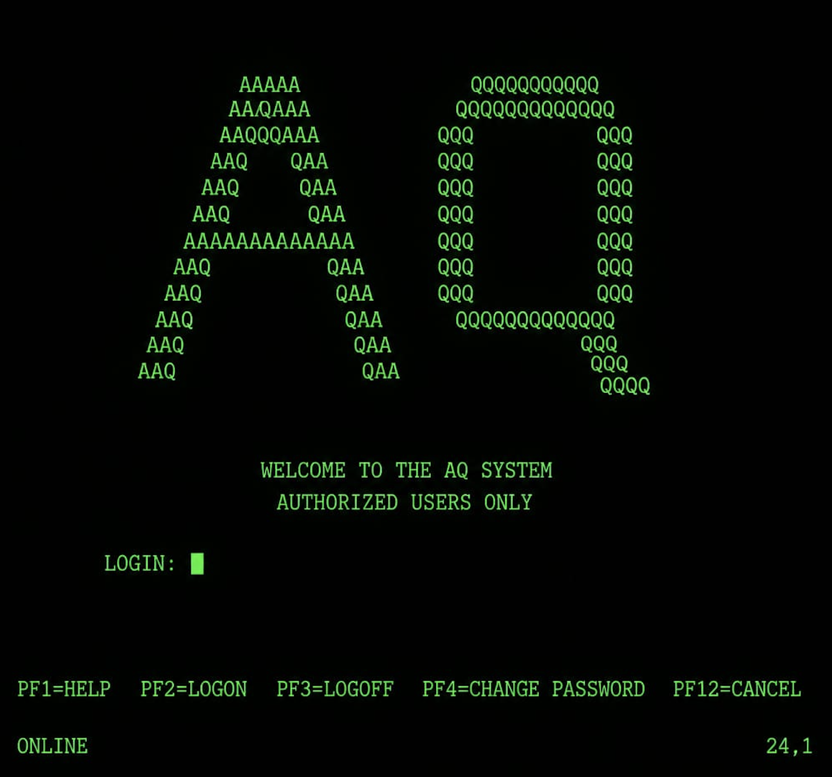
Resource Link PL/SW Live Demo sw-embed.github.io/web-sw-cor24-plsw PL/EDIT documentation docs/pl-edit.md Mass Compile documentation docs/mass-compile.md Video walkthrough (YouTube) youtube.com/watch?v=9KQ3ohU4BHE PL/SW (the language) sw-embed/sw-cor24-plsw Web demo source sw-embed/web-sw-cor24-plsw Prior posts TBT #9: UNIVAC Startrek, TRS-80 Adventures, and COR24 BASIC · Bucket List #3: Mass Compile + PL/EDIT context Comments Discord The AQ Setting
AQ ran on MVS/ESA. From the user’s seat, every interaction was a 3270 block-mode terminal: you didn’t type interactively the way you do at a modern shell — you filled in fields on a screen, pressed Enter (or a PF key), the entire screen went to the host, the host processed it, and a new entire screen came back. Round-trip latency was small only by the standards of the day. The medium shaped the workflow.
Hundreds of developers shared this system. They edited PL/X (IBM’s internal PL/I dialect, used for systems work and OS components) and System/370 assembler. They submitted batch compile jobs to JES2. They scheduled printouts (yes, printouts — a real cabinet of green-bar paper down the hall) or browsed compile output online. The two universal pain points of every developer’s day were:
- Authoring is slow because most of what a working programmer types every day is repetitive boilerplate — IF/ELSE framing, DO/END loops, DCL declarations, PROC headers, MACRODEF blocks — and the editor gives you no help avoiding it.
- Turnaround is slow because submitting a compile job means joining a queue, and on a busy day that queue could be an hour long. By the time results came back, you had context-switched to a different program four times.
Two colleagues built tools to push back on each of those. They were exactly the kind of internal productivity tooling that did not exist as products on the open market in 1985 — IDEs were a Macintosh / Smalltalk lab curiosity, Emacs existed but was a Unix-room thing not a mainframe thing, and the average corporate mainframe shop ran whatever editor IBM happened to ship. Internal tools filled the gap, and the good ones spread by reputation.
PL/EDIT — Templates Before They Were a Word
A colleague (whose name I am withholding here, since I have not asked their consent to publish it forty years on) wrote PL/EDIT. The premise was simple: most of what a PL/X programmer typed was boilerplate. The first three lines of every IF block. The DO/END framing of every loop. The DCL statements at the top of every record declaration. The PROC header with its parameter list and RETURNS clause. The MACRODEF blocks. None of it was creative work. All of it was syntax.
PL/EDIT replaced character-by-character authoring with trigger-driven template expansion. You typed a short trigger like
IFand pressed F4, and the editor expanded the trigger into a full IF/ELSE block with named fill fields. You pressed Tab to advance through the fields, Shift-Tab to go back. F4 cost one extra round trip to fetch the expanded screen, and the trade was easy: a few characters of trigger plus one round trip, in exchange for not typing the dozen-plus characters of boilerplate by hand.The triggers covered every form a working programmer touched dozens of times a day — IF/ELSE blocks, DO WHILE and counted DO loops, SELECT/WHEN dispatch, scalar and record declarations, PROC headers with parameter lists and return types, CALL and RETURN, inline-assembler blocks, the macro-definition forms used for code generation. A help button opened the active trigger list; a Format button re-indented block structure that had gotten ragged.
This is exactly the model that snippets, IDE templates, and YAS-snippet would later mainstream in the 1990s and 2000s. PL/EDIT did it in the mid-1980s. It was not the first template editor anywhere — TECO and Emacs had abbrev-mode, and similar systems had snippets — but it was the only one that hundreds of us had access to, and the productivity difference between using it and not was night and day.
PL/EDIT on COR24 PL/SW

The COR24 PL/SW live demo is a Yew/WebAssembly application that hosts the PL/SW compiler, COR24 emulator, and a small source editor entirely in the browser. PL/EDIT is implemented there as a hotkey-driven editing mode you toggle with the
PL/EDITbutton in the editor header. The mechanism is faithful to the original idea: type a trigger, press F4 (orCtrl+Space), and the trigger expands into a template with fill fields.Tabadvances through fields;Shift+Tabgoes back;Ctrl+Enterinserts a newline inside block content.The PL/SW source-editor trigger set:
Trigger Expansion IF/IFSIF/ELSE block; single-statement IF DW/DODO WHILE; counted DO SEL/WHENSELECT/WHEN dispatch; WHEN branch DCL/REC/BASEDscalar / level / BASED record declaration P/PR/NAKPROC; PROC with RETURNS; OPTIONS(NAKED) PROC ASMASM DO block (inline assembler) CALL/RET/RETV/GCALL; RETURN expression; void RETURN; GOTO Plus a complementary set for
.mswmacro-include files (a PL/SW invention —.mswis the PL/SW analogue of a header file with macro power):MDfor MACRODEF,REQ/OPTfor required/optional parameters,GENfor GEN DO blocks,INCfor%INCLUDE,INVfor invocation. The?button shows the active trigger list.Formatdoes PL/I-style re-indentation of block structure (PROC,IF/THEN/ELSE,DO WHILE, countedDO,SELECT/WHEN/OTHERWISE,ASM DO,GEN DO,MACRODEF, multi-lineDCLrecords). Full reference in docs/pl-edit.md.Mass Compile — Submitting Jobs for Programs You Had Not Written Yet
A different colleague tackled the turnaround problem with Mass Compile.
The naive workflow on AQ went: edit a program, save it, submit a compile job, wait. The wait could be five minutes; it could be an hour. Whatever the wait was, you context-switched, and when results came back you context-switched back. If you had a stack of related changes across several programs, you submitted them serially — finish program A, submit, wait, switch to program B, edit, save, submit, wait. The queue and the editor were unsynchronized: time you spent editing was time the compile queue was not running on your behalf.
Mass Compile was a screen — a single 3270 panel — where you could schedule a batch of compile jobs in advance. The trick the screen made possible was the one I still find astonishing: you could submit compile jobs for programs you had not written yet. The compiler did not know that. The compiler did know that when its turn arrived in the queue, it would go look up the named source member in the editor’s working storage and compile whatever was there at that moment. So:
- You scheduled jobs for programs A, B, C, D — four compiles, queued in order.
- While the queue waited for A’s slot to open, you finished editing A.
- While A was compiling, you finished editing B.
- While B was compiling, you finished editing C.
- While C was compiling, you finished editing D.
The queue and the editor were now synchronized: every minute the queue spent moving forward was a minute the editor spent moving forward. The total wall-clock time to compile four related changes dropped from “four queue-waits in series” to “one queue-wait plus four edits in parallel with three compiles.”
The catch was the file lock. The editor held an OS-level file lock on each source member while you were editing it; JES2 needed the same lock to read that source when the compile job reached the head of the queue. If your job got there before you finished editing, JES2 waited on you. Messages would scroll into the bottom of your screen telling you, then telling you more emphatically, that a compile job was blocked waiting for your editor to release the lock. Senior engineers learned the social cost of holding the queue on a busy day; you did not want operations or your manager to start wondering why nobody else’s compiles were moving.
This was, in its own way, the first JIT-style “compile under pressure” workflow I ever saw. The compile job did not block on the source being final at submit time. The source was final as of the moment JES2 acquired the file lock, not as of submission. Speculative scheduling, OS-level file-lock arbitration, and a small dose of social pressure to keep you honest. The trick has not really gone away — modern build systems (Bazel, Buck, Cargo) all have variations on “kick off compute against the inputs as soon as they stabilize,” and CI systems do something analogous with branch-based job queues. But none of them show you the queue moving the way the AQ Mass Compile screen did.
Mass Compile on COR24 PL/SW
The COR24 PL/SW live demo has no JES2 and no OS-level file locks — it runs entirely in WebAssembly with the compiler and emulator embedded in the page. What the demo does preserve is the speculative-scheduling shape and the queue-vs-edit pacing, recast as a homage rather than a faithful port.
Open the dialog from the source editor’s action row. The left panel is a job list; you add rows, pick demos, optionally edit per-row scratch source, then
Submit(one row) orSubmit All(every row). Jobs run sequentially through the statesqueued→compiling→assembling→running→complete(orfailed). Submitted jobs do not modify the bundled demo source; they compile from browser drafts. If a queued job has no scratch edit, it snapshots the current draft for that demo when the job enters thecompilingstate, not when the job is queued. So you can keep editing program A while program B is compiling.The lock-in-spirit is the
waitingstate. If a queued job reaches the head of the queue while its scratch editor is still dirty (you have not pressedSave), the job state changes towaitingand the queue stops there until you save. That is not a file lock; it is a save-vs-unsaved sentinel. The mechanism is different from JES2’s; the role it plays is the same — the queue does not move until your edit is committed.Full reference in docs/mass-compile.md.
Why These Two Keep Coming Back
PL/EDIT and Mass Compile are about making each interaction with a slow system carry more weight. PL/EDIT trades a single F4 round trip for a dozen-plus characters of typing you would otherwise do by hand; Mass Compile lets the queue move while you keep editing. Both are productivity multipliers in environments where the dominant cost is wait time.
I keep finding the same shapes today, in different surfaces:
- Snippets and LSP scaffolds in modern editors are PL/EDIT’s children: type a trigger, get a templated form with fill fields. Same idea: stop typing the boilerplate, fill in only the parts that change.
- CI parallelism, build queues, and content-addressed caches are Mass Compile’s children: do not block on the source being final at submit time; do the expensive thing as late as possible against whatever inputs are stable; let the queue move forward in parallel with editing. sw-launcher’s cache-key formula is a content-addressed version of the same idea — the work runs against the inputs that exist when it runs, not when it was scheduled.
- AI agents working from a queue of tasks are Mass Compile’s grandchildren: submit a sequence of work items; let the agent process them while you keep going; surface warnings when an item is blocked on input you have not provided yet.
The 1980s mainframe shop was not primitive. It was constrained — a different set of constraints than today’s, but the people working in it solved their constraints with surprising elegance, and the productivity tooling that survived from that era keeps re-emerging in modern surfaces because the underlying problems — slow authoring, slow turnaround, queue contention — have only changed in detail. The medium changes; the moves stay.
If you have a few minutes, the live demo is worth poking at. Type
IFand press F4. Open Mass Compile, add a few rows, edit one of them while the queue runs ahead. The 3270 is gone; the workflow is intact.Login
AUTHORIZED USERS ONLY. ONLINE 24,1.Part 10 of the Throwback Thursday series. View all parts
Comments or questions? SW Lab Discord or YouTube @SoftwareWrighter.
-
2876 words • 15 min read • Abstract
Bucket List #3: 3D Source Code, Five New Languages, and Visible Compilers

Why this matters — A bucket list is only useful if it grows as fast as it shrinks. Crossing things off without adding things back is how a list gets shorter than the curiosities of the person carrying it. The three categories below are what’s been quietly moving from “interesting” to “I’m actually doing this” since the last post — and they share a thread: each one is something a working engineer rarely gets to do (build a new programming language, sculpt a new authoring surface, or instrument a compiler so you can watch it think) because the day job never gives that kind of room. Retirement and AI agents jointly do.
Resource Link DiscoveryOne (3D source) softwarewrighter/DiscoveryOne Tuplet (2D, DiscoveryOne’s predecessor) softwarewrighter/tuplet sw-MLPL (array language) sw-ml-study/sw-mlpl · live REPL PL/SW (PL/I-inspired systems lang) sw-embed/sw-cor24-plsw · live demo SWS (Tcl-like resident shell) sw-embed/sw-cor24-script Bucket List softwarewrighter/bucketlist Prior posts Part 1 · Part 2 Comments Discord Source Code’s Third Dimension
Programmers get attached to the medium they happened to learn on. People who started on punch cards remember source as a one-dimensional thing: a stack of cards, fed sequentially, each card eighty columns of fixed-width sequencing, each program a literal physical pile. People who started on glass terminals (which is most of us) think of source as two-dimensional: a window of lines and columns, scrollable in two axes, with the assumption that the meaningful structure lives inside that rectangle.
Every editor we use today is still a 2D-rectangle authoring surface. We have learned to interleave many concerns inside that rectangle — the algorithm, the types of inputs and outputs, the preconditions and postconditions the algorithm assumes, the generated form the compiler ends up emitting, the implementation layers (logging, error handling, instrumentation) that production code accumulates. Modern languages provide affordances for hiding most of this — type signatures collapse, comments fold, error handling moves to attributes or decorators — but it all still lives in the same rectangle, fighting for the same screen real estate, and the front-of-the-eye reading order is whatever the editor’s vertical scrollbar decides.
Punch cards are 1D. Screens are 2D. What if source were 3D?
DiscoveryOne is the project I am sketching to make that question concrete. Every glyph in a DiscoveryOne program has an
(x, y, z)coordinate and an aspect label drawn from a fixed set:@front,@left,@right,@top,@bottom,@rear,@internal. A definition is not a block of text; it is a small cube of meaning, and the user views one facet at a time:Facet Role Front Algorithm gist — the readable story Left Inputs (arity, names, types) Right Outputs (arity, names, types) Top Preconditions Bottom Postconditions Rear Generated form (WAT or stack IR) Internal Implementation in spatially-separable layers The Yew/WASM web app loads the file, projects it onto the requested facet, and runs the WASM module in-page when you click Run. A
*Powerdefinition readingn e -> p; p <- 1; loop e times: p <- p * nlives on@front;n : Int, e : Intlives on@left; the output typep : Intlives on@right;e >= 0lives on@top;p == n^elives on@bottom. Aspects (preconditions, postconditions, tracing, profiling, error recovery) live on spatially separate@internallayers so the front facet stays uncluttered for reading.DiscoveryOne is the successor to Tuplet, my current 2D-layout-sensitive language with first-class named tuples and user-mintable verbs (the
*operator literally mints new syntax). Tuplet keeps source 2D but layout-sensitive — where a glyph sits on a 2D grid changes its meaning. DiscoveryOne is the next jump: from “layout matters” to “facet matters.” The same glyph in two different@-aspects participates in two different parts of the program’s meaning.Whether 3D source is useful is a real question. It might turn out that the seven facets are too many, or that the projection UI is too clumsy, or that humans really do read code best as a flat top-to-bottom story. I don’t know. The way to find out is to build it, drive a non-trivial program through it, and see whether reading the front facet of an unfamiliar definition is faster than reading the equivalent flat code with all its types and contracts and tracing inline.
DiscoveryOne is currently pre-M0 — the specification is committed; no code yet. The single demoable target (M7 in the saga plan) is one vertical slice: the user authors a
*Powerdefinition and a*syntax do _ while _ end expandsyntax declaration, and runs both inside the web app. If that slice feels right, the rest follows.Five Languages of My Own, in Flight
The other thing on the list right now is making programming languages, plural. Five of mine are currently between “design committed” and “live demo,” each picking a different point on the build/run space. Listed in roughly the order I started them:
PL/SW — PL/I-Inspired Systems Language
sw-cor24-plsw is a small systems-programming language inspired by PL/I (and a little IBM HLASM). It is the language I use to write higher-level COR24 programs — the SNOBOL4 interpreter, parts of the toolchain, the Fortran compiler in flight. It compiles natively to COR24 assembly and has its own vibe-maintenance heatmap of issues closed in the past few weeks (forty-plus, including the inevitable parade of “AST pool too small,” “MAX_PROCS too small,” “emit buffer too small” capacity bumps).
PL/SW’s interesting bet is macros: PL/I-style
%DEFINEandMACRODEF GENblocks that emit assembly. That makes the language usable as a meta-assembler — a higher-level surface that still gives you bit-level control over the COR24 instruction stream. It is the language I would have wanted in 1985 if I had had any say in the matter.SWS — Tcl-Like Resident Shell
sw-cor24-script is a tiny Tcl-style scripting language that runs inside the resident monitor on COR24, sharing the program registry. The shell is a single binary that loads at
0x020000(above the monitor at zero), and its commands operate on whatever programs the monitor has loaded into the slot table. It is the missing surface for a “1980s style” embedded workflow — the user typesrun helloat a prompt, the monitor’s service vector dispatches into the program at that slot, and control flow returns through a longjmp-style trampoline.SWS exists because every other language in the lab is non-resident — a load happens, a program runs, the run ends, the host runs the next thing. SWS is the language designed for the case where the user is part of the loop: type, run, observe, type again. The repl on a 1 MiB COR24, with a 3 KiB EBR stack, in the year 2026.
sw-MLPL — A Rust-First Array Language
sw-mlpl is the array-and-tensor programming language I am building for the ML side of the bucket list. The lineage is APL → APL2 → J → BQN, but the implementation is Rust-first: a REPL in the terminal and the browser, a
mlpl!proc macro that lets MLPL expressions live inside Rust source, anmlpl buildpath that compiles MLPL programs to native binaries, and a roadmap of backends (Apple MLX for Apple Silicon, CUDA for distributed training, Ollama / llama.cpp / OpenAI-compatible servers for LLM glue).MLPL is the only one of the five that is mostly built — the live REPL works in the browser today, the language reference is written, the compiler implementation has a tour document for educational reading. What’s still ahead is the long tail of array-language features (rank polymorphism, fork composition, J-style tacit programming) and the big backends. It is the language I will use to do the fine-tune-a-base-model item from part 1.
Tuplet — 2D Layout-Sensitive Language with Mintable Verbs
tuplet is the language I am driving as my main daily-language experiment. It is 2D-layout-sensitive (where a glyph sits on a grid matters), has first-class named tuples and multi-output verbs, and lets the user mint new verbs and new syntax via the
*operator. The kernel is small; everything else — including control flow — is library code expressed in the kernel. The host is an OCaml-subset interpreter; the runtime target is Forth running on the COR24 emulator.Tuplet is currently in the “wakes the dragons” phase of language development — the language compiles, demos run, but the OCaml interpreter underneath has been thrashing its heap until the GC work in flight (
sw-cor24-ocaml#28) lands. Once that lands, Tuplet’sheap_limitshould shrink, not stay where it is, and the language will start to feel less fragile.DiscoveryOne — 3D Successor
Already covered above. DiscoveryOne is to Tuplet what Tuplet is to a flat language: one more dimension of authoring surface, one more affordance for separating concerns spatially rather than syntactically. It is the place where I get to ask the broader question — can authoring be 3D? — without bolting it onto a language whose users are already doing real work.
The 1980s Ancestors: Mass Compile and PL/EDIT
Two of the threads above have ancestors I worked on as a junior engineer at IBM in the 1980s — Mass Compile, a screen for scheduling batch compile jobs in advance (including jobs for code you had not finished writing), and PL/EDIT, a template-driven editor that expanded triggers into boilerplate via hotkey. Both ran on AQ, an MVS/ESA time-sharing service. The Throwback Thursday post tells the story in detail. The reason they come up here is the conceptual lineage: Mass Compile’s “do the expensive thing against whatever inputs are stable when it runs” is the same shape as sw-launcher’s content-addressed cache, and PL/EDIT’s “fill in the slot that matters and let the template handle the rest” is the same shape as DiscoveryOne’s facet authoring. Both ideas keep coming back, in different shapes, every time the dev loop gets a new bottleneck.
I maintained both tools; I did not write them. That was the right level for me at the time, and the vibe-maintenance post reprises the lesson forty years later: a tool you maintain long enough teaches you the design choices its author made and the seams where the next idea wants to break in. The bucket list, on this reading, is partly a list of the bottlenecks I have seen over the years and the surfaces I want to build to push back on them.
Visible Compilers — The Missing Tool Category
The unifying gap, behind all of the above, is visibility.
Almost every CS curriculum spends a semester on compilers. Almost every working engineer uses one every day. Almost no engineer has ever watched a compiler run — watched the lexer turn a stream of characters into tokens, watched the parser grow an AST, watched a type checker fail and recover, watched a register allocator color a graph, watched a heap fill up and a GC reclaim it. The mechanism is invisible. We read about it. We trust the diagrams in textbooks. We never see the diagram move.
The next chunk of the bucket list is the tooling that fixes that. For each of the five languages above (and ideally for the COR24 toolchain in general), I want a visible counterpart:
Step-Through Lexer
A panel that shows the source on the left and the token stream on the right. Click “step” — the cursor advances by one token, the new token glows in the right panel, the consumed characters fade in the left panel. Speed it up to “auto” and the whole stream animates past at one-token-per-50ms. See the lexer.
Animated Parser
The same idea for the parser: source on the left, the AST growing on the right as a tree. Each shift / reduce step is a step. The current rule highlights. The error recovery, when it happens, is visible — a subtree dies, a new one grows in its place, the resync token is annotated.
AST Viewer with Types Folded In
A static view (not animated) of the AST after the parser finishes, with type annotations folded into each node. Hover over a node to see its full type; click to dive into a subtree. The same view, but for the typed AST after the type checker runs, with inferred types added. Then the same view for each lowering pass — AST → CFG → SSA → linearized IR — with arrows showing what produced what.
Lowering and Codegen Side-by-Side
Three columns: source, IR, target assembly. Pick a line in any column; the corresponding range highlights in the other two. The lowering passes get their own animation: tail-call elimination shows the call disappearing and the branch appearing; closure conversion shows the free variables being collected and packed; trampolining shows the indirect jump being inserted.
Register Allocation, Visualized
The conflict graph. The live ranges. The interference. The spills. Watch the graph-coloring algorithm run, color by color. Watch the spill heuristics pick which range to evict. See what your compiler optimizer is actually doing when it picks
r4instead ofr2for that loop variable.Simple Optimizations Before/After
Constant folding. Common subexpression elimination. Dead-code elimination. Loop-invariant code motion. Each one as a side-by-side before/after with the moved/removed code highlighted. The whole point of these is that they’re small and understandable if you can see them; they’re black-box magic if you can’t.
Heap and Stack Instrumentation
A live memory map. The stack growing and shrinking with each call/return. The heap filling with allocations, each allocation a colored block. Free / dispose / reclaim animates: the block fades, the free list pointer redirects, the block is gone. The hardest classes of bug — use-after-free, double-free, leaks — become visible the moment the memory map is.
Garbage Collectors at Work
Mark-and-sweep, copying, generational. Each one a different animation. Mark-and-sweep: a wave of color sweeps the heap from the root set; everything not colored gets reclaimed. Copying: two semi-spaces, the live objects walk from one to the other, the old space is wiped. Generational: nursery / tenured, promotions visible, write-barrier hits flagged. The OCaml interpreter’s incoming GC (sw-cor24-ocaml#28) would be the first candidate — I want to watch it run.
JITs Tiering Up
A function getting called once: interpreted. Called a thousand times: tier-up triggers, a jitter compiles a baseline native version, the call site rewrites itself, subsequent calls run at native speed. Hit a deopt: tier-down to the interpreter, the native code gets discarded, the next thousand calls retrigger the jit. This is the part of modern runtime engineering that is hardest to see; the visualization that makes it watchable would be the tool I would have wanted as a junior engineer.
The pattern across all of these: the textbook diagrams are static. The visualizer shows them moving. Once you have seen a register allocator color a graph, you cannot read about register allocation the same way again — the diagrams in the textbook map onto something you actually watched happen.
Why Now
All three categories above became viable in the same window for the same two reasons — retirement gave the time, AI agents gave the reach. Every one of these projects, on its own, would have been a multi-year team effort five years ago. Today they sit on the list, and the list is moving:
- A new paradigm of programming-language surface (DiscoveryOne) is one vertical slice (M7) from being demoable.
- Five language implementations sit between “compiles” and “in production daily use,” each filling a different niche in the small ecosystem.
- The visible-compiler tool category is the unifying frame — the surface I want to have for every compiler I write, including the five above.
The next post in the series will probably be about whichever of these turns out to land first. My money is on the lexer / parser visualizer for sw-MLPL, since the language is already runnable and the visualizer is mostly “yew web app” away. We’ll see.
The list keeps growing. The bucket keeps filling. That’s the point.
Part 3 of the Bucket List series. View all parts
Comments or questions? SW Lab Discord or YouTube @SoftwareWrighter.
-
2523 words • 13 min read • Abstract
Personal Software #9: Vibe-Maintenance --- When AI Agents Don't Just Write Code, They Fix Bugs

Why this matters — “Vibe-coding” gets the headlines because it produces something visible: a new feature, a new demo, a new tool. Vibe-maintenance is the quieter half. It does not show up as a flashy commit message; it shows up as a green “Try it” badge that used to say “In dev,” or as a closed-issues heatmap that is busier than the commits one. If your only frame for AI-assisted development is “the agent writes new code,” you miss the half of the work where the agent is reading existing code, finding the assumption that was wrong, and patching it. Almost every senior engineer who has tried to use AI agents finds maintenance more useful than greenfield work; the post argues for why, and what the human still has to do.
Resource Link Status dashboard sw-embed.github.io/web-sw-cor24-demos/#/status Demos repo sw-embed/web-sw-cor24-demos Closed-issues report (raw) reports/closed-issues.html Prior Personal Software post Personal Software #8: sw-launcher — One Ring to Rule Them All Related AI Tools post AI Tools #3: sw-checklist — Reining In AI Coding Agents Comments Discord The Corollary to Vibe-Coding
Vibe-coding, as the term gets used: a human describes intent, an AI agent writes the code, the human accepts or redirects. The implicit assumption is that new code is the bottleneck. For a greenfield project, sure — there is nothing to maintain because there is nothing to maintain yet. For a lab whose accumulated output now spans 37 repositories — assemblers, emulators, cross-compilers, p-code VM, native interpreters for BASIC and Forth and APL and Smalltalk and Macrolisp and SNOBOL4, host tooling, the resident-shell trio, web demos for most of them — the bottleneck moved a long time ago. New code lands; new code interacts with old code; old code that was fine on its own now has a corner that nobody exercised; an issue gets opened.
Vibe-maintenance is the same loop with a different verb. The human writes an issue title. The agent reads the relevant code, locates the assumption that was wrong, makes a minimal patch, adds a regression test, and closes the issue. The human’s job is not to write the code; it is to write the issue with enough specificity that the agent has somewhere to start, and to read the diff with enough care that the test does not just pin in the bug under a different name.
The skill the human keeps is not “writing code.” It is symptom description.
The Status Tab as Visualization
web-sw-cor24-demos is the landing page for the COR24 ecosystem. Its Status tab makes the lab’s operational state visible at a glance:
- A 37-row table of every repo with a colored badge — “Try it” (green), “In dev” (yellow), “In plan” (orange), “Future” (red), “n/a” (neutral) — for repo readiness, web-UI readiness, and AgentRail saga presence.
- An issue chart per repo: open vs. closed counts and a sparkline.
- A Closed Issues by Repo & Date heatmap, generated by
scripts/gen-closed-issues.shfrom the GitHub API. - A Commits by Repo & Hour heatmap, the same shape one row down.
- A “Gaps” panel calling out the cross-cutting work the lab has not yet done (software floating-point library, native COR24 C compiler, etc.).
The headline number on the closed-issues chart, at the time of writing: 28 repos, 141 issues, 18 days. Eight closed issues a day, sustained, across two dozen active repos. That is not an output a single human writing code by hand achieves. It is also not an output a single human reviewing AI-written code achieves if every issue requires a fresh greenfield design — it is only achievable because most of those 141 issues were bugs in code that already existed, and an agent can fix one of those in a fraction of the time it took to write the original.
The two heatmaps next to each other tell a story: the commits chart shows when work happened (clusters in the morning, fewer at night, weekend bursts when an idea hit); the closed-issues chart shows what work settled (each cell is a problem that has a regression test guarding it). The cells are mostly numbered links, so any cell on the chart is one click from a real PR diff. That traceability is the whole point.
Four Patterns of Vibe-Maintenance
Reading down the closed-issues report by category — not by repo — four kinds of fix dominate.
1. Capacity-Limit Bumps
The numerically-largest category. A compiler or interpreter has an internal table whose size was guessed at first commit (
MAX_PROCS = 32,INPUT_BUF_SIZE = 8192, AST pool of 256 nodes, emit buffer of 32 KiB, string literal table of 32 entries). A real program hits the limit, the agent bumps it, and a follow-up issue raises it again later when an even bigger program lands.A small sample, all closed in this window, all from
sw-cor24-plswandsw-cor24-pascal:- “AST pool exhaustion (256 nodes) causes misleading parse errors.”
- “Source buffer (8 KiB) too small for larger programs.”
- “Emit buffer (32 KiB) too small for programs with large static data.”
- “DEF_MAX (32) too small — %DEFINE silently dropped when exceeded.”
- “Global symbol table limited to 64 entries (SYM_SCOPE_MAX).”
- “Raise MAX_PROCS from 32 to support larger programs.”
- “Raise MAX_STRINGS limit from 16 to support larger programs.”
- “Raise INPUT_BUF_SIZE from 32768 to support larger programs (third bump).”
Each one is a one-line const change plus a regression test that compiles a representative-sized input. The third-bump issue is the funny one: the limit is no longer a guess, it is a parameter that grows with the corpus. Eventually the right answer is “the table grows dynamically,” but the lab’s working assumption is that bumping a static limit is a one-cycle fix, while a dynamic table is a one-day refactor that earns its keep only after the same limit has been bumped enough times to justify it. The ratchet is the right tool for this kind of debt.
2. Subtle Codegen Bugs
The most interesting category. These are not “the feature is missing”; these are “the feature is silently wrong.” A few from the same window:
sw-cor24-plsw#8: “BYTE field reads use signedlbinstead of unsignedlbu.” A one-instruction error; values 128–255 sign-extend to negative integers, breaking pattern matching and arithmetic.sw-cor24-plsw#31: “Function return corrupts r1 -> jmp to PC=0 (programs that call PUT_DEC re-enter_start).” A clobbered callee-saved register; the symptom looks like an infinite loop with the program re-running from the top.sw-cor24-pcode#10: “p24-load: patch_code_relocations incorrectly relocates negative push literals.” A pointer-vs-immediate confusion in the linker; small negative integers get rewritten as garbage addresses.sw-cor24-x-tinyc#19: “Codegen: integer division with negative dividend returns wrong result.” The C cross-compiler’s sign-handling.sw-cor24-snobol4#13: “Arithmetic on a pattern-captured string returns garbage on first use.” A type-tag bug in the SNOBOL4 interpreter’s value union.sw-cor24-pascal#16: “write(chr(n))outputs integerninstead of character.” Built-in dispatch on the wrong type.sw-cor24-basic#1: “ABS function silently returns wrong value (parsed as variable A).” The lexer treatsABSas a variable rather than a builtin, soABS(-3)parses as(A) * BS * (-3)— a beautifully evil bug whose title carries the entire diagnosis.
These are the issues where vibe-maintenance shines. Each title is a complete reproducer in plain English. The agent reads the title, opens the relevant translation unit, finds the wrong instruction or the wrong dispatch, fixes it, writes a one-program regression test, and closes the issue. The human never wrote a line of code; the human wrote a fifteen-word symptom description.
3. Surface Language Features Rolling In
Each language interpreter ships with a minimum viable feature set, and demos that exercise more of the historical language drag in features that didn’t make the first cut:
- BASIC: DIM integer arrays, DATA / READ / RESTORE, ON expr GOTO/GOSUB, MOD, bitwise BAND/BOR/BXOR/SHL/SHR, CONT after STOP. (
sw-cor24-basic#2..#7.) - OCaml: top-level let bindings, multi-line match expressions, mutable refs, records, list combinators (
map/fold_left/filter), char literals, block comments, exceptions. (sw-cor24-ocaml#3..#11.) - Forth: forth-in-forth gets DO/LOOP, ?DO, WHILE/REPEAT, AGAIN, CONSTANT, VARIABLE, hashed dictionary;
:NONAME. (sw-cor24-forth#1..#5.) - SNOBOL4: SIZE/SUBSTR/CHAR builtins, pattern-replacement assignment, case-preserving INPUT mode. (
sw-cor24-snobol4#1..#10.) - TinyC: goto + labels, compound literals, designated initializers,
_Noreturn,restrict,inline, octal literals, multi-dimensional array declarations. (sw-cor24-x-tinyc#2..#11.)
Each of these is the kind of feature that would take a human a half-day if they had to read the existing parser, find the right place to extend it, and add the right test fixtures. Vibe-coding compresses that to a half-hour of agent work plus a human-written acceptance criterion. The acceptance criterion is the part that does not get cheaper.
4. Cross-Cutting Tooling Bugs
The last category is the meta one: the tooling that generates the dashboards itself has bugs. A representative pair from the demos repo’s commit log, just in the past two weeks:
fix UTC-to-local date conversion in gen-issue-chart, rebuild and deploy pagesfix timezone in activity reports: convert UTC dates/hours to local, regenerate tables
Two separate “use Local::now() instead of Utc::now()” commits in two different generators. The cells in the heatmap were shifted by a few hours, which made yesterday’s work look like today’s, which made the dashboard wrong — subtly, in a way that would only catch the eye of someone who knew what they had committed yesterday. The agent fixed both. They are listed in the dashboard the agent generated. The fact that the dashboard works is itself a regression test on its own generators.
The Skill That Doesn’t Go Away
Every category above leans on the same human contribution: a precise description of the symptom, often as the issue title.
Compare the two SNOBOL4 issues:
#1: “Missing string builtins: SIZE, SUBSTR, CHAR return 0 for all inputs.”#11: “OUTPUT corruption: concat-OUTPUT in a loop truncates when a different block declares a pattern-match with:F(forward_label).”
Both are real titles. Both are diagnoses, not just symptoms — they tell the agent exactly what subsystem to read.
#1is mechanical: open the builtins table, see that the entries return 0, fix them.#11is forensic: the title names the loop, the operator, the block, the directive, and the conditional — the agent has the entire reproducer one paste away from a test fixture.The bad version of either title would be “OUTPUT is broken.” That title costs the agent half its budget on guessing what “broken” means and produces a fix that may or may not address the real bug.
The skill the lab keeps practicing is writing the issue at the level of detail the agent needs. That is roughly the same skill an engineer uses to file a useful bug report against another engineer. The difference is that the audience is faster and cheaper than the engineer; the title is read inside a second, the diff is back inside a minute, and the regression test is attached. The economics of writing good issues, in a vibe-maintenance world, are vastly more favorable than they were when the audience was a human queue with their own backlog.
The Feedback Loop

The maintenance loop, as it actually runs in this lab, has five steps:
- Symptom. A demo, test, or build fails. A user reports a wrong output. A regression test caught a regression. CI flagged a gate.
- Issue. The human (or another agent) writes a one-line title and a short body that names the conditions. Most of the time the title is enough.
- AgentRail saga step. For non-trivial fixes, the work goes onto an AgentRail step — a single session does the diff, commits, and runs
agentrail complete. The session is bounded; the next session is for the next step. - Regression test. The diff includes a test that pins the bug fixed.
cargo test/make testis the contract. If a future change re-introduces the bug, the test catches it. - Status refresh.
cargo run -p gen-statusand the closed-issues / commits scripts re-pull from the GitHub API; the heatmap moves; the badge in the table tilts greener.
This is not a novel workflow — it is what every well-run engineering team does. What is new is that the per-issue cost is small enough that the heatmap is busy. Eight issues a day across a constellation of personal projects, sustained for weeks, is the kind of cadence that used to require a small team. One human plus AI agents plus the discipline of writing good issues hits it.
The artifact, in the end, is not “the AI fixed 141 bugs.” The artifact is the dashboard — 28 repos getting visibly greener, with each cell on the heatmap a clickable link to the diff that closed it. The lab is legible, and being legible makes it possible to do the work at this pace in the first place.
Where It Sits in the Personal-Software Toolkit
sw-checklist keeps the shape of the code in line. sw-launcher keeps the shape of the load plan and memory budget in line. AgentRail keeps the shape of the work in line — one saga, one step at a time, with a faithful audit trail. The Status tab is the operational dashboard that makes the result of all three legible at a glance. None of those tools, individually, would be enough to keep a 37-repo lab maintainable by one person; together they make vibe-maintenance the steady-state mode of operation.
The car is up on the lift. The mechanic is not building anything new today. The mechanic is going around with a torque wrench, an oil drain, and a parts list, and at the end of the afternoon every gauge is in the green again. AI agents do not change which afternoons that work happens on. They change how many cars fit in the shop.
Part 9 of the Personal Software series. View all parts
Comments or questions? SW Lab Discord or YouTube @SoftwareWrighter.
-
4405 words • 23 min read • Abstract
Personal Software #8: One Ring to Rule Them All --- sw-launcher's Memory Profiles, Heap Budgets, and a Working Scenario A

Why this matters — AI coding agents working across multiple sw-embed repos do not have the patience or the pattern-matching to get the load plan right by inspection. They will happily write
cor24-run --load-binary out.bin@0 --load-binary app.p24@0x10000 --patch 0x12=0x10000 --entry 0from scratch every time, sometimes inventing flags that don’t exist. The fix is not better agent prompts; it is removing the freedom to invent.sw-launch run <scenario>is the only verb the agent gets, the TOML is the only place memory-layout decisions live, and the schema makes oversized heaps argue for themselves before the validator accepts them.Resource Link Repo sw-cli-tools/sw-launcher 13-repo survey docs/survey/index.md · schema-gaps.md Memory stance docs/memory-stance.md · docs/heap-analysis.md COR24 emulator sw-embed/cor24-rs Driven projects sw-cor24-pcode · sw-cor24-ocaml · sw-cor24-pascal · sw-cor24-basic Related AI Tools post AI Tools #3: sw-checklist — Reining In AI Coding Agents With a Code-Metrics Ratchet Comments Discord The Problem: Every Language Has Its Own Loader
The COR24 is a 24-bit machine with 1 MiB of SRAM, a 3 KiB EBR hardware stack, and an MMIO aperture at
0xFF0000. The host-sidecor24-runemulator accepts a small surface —--load-binary path@hex_addr,--patch hex_addr=hex_value,--uart-input "...",--entry,--speed,-n— and that’s the universe.What changes between repos is what gets loaded where, which runtime word has to be patched to point at the layer above it, and how source and data ride the UART. The Phase 0 survey looked at thirteen working repos and aggregated the patterns. A few from the comparison table:
repo loads patches UART src UART data heap stack approx SRAM basic 1 0 yes no emb hw EBR ~64 KiB forth 0 0 yes no emb hw EBR ~256 KiB macrolisp 0–1 0 yes snapshot emb hw EBR ~512 KiB ocaml 2 2 yes post-EOT emb+res emb in pvm ~512 KiB pascal 1–2 1 yes no emb emb ~64 KiB plsw 0 0 yes no emb hw EBR ~1 MiB snobol4 1–3 0 yes mode-flag emb emb ~128 KiB monitor many 0 no no emb hw EBR ~64 KiB tuplet 3 2 yes image@0x080000 res emb in pvm ~768 KiB Every project’s
scripts/run-*.shre-encodes one of these shapes. None of them validate. None of them cache. None of them notice when the OCaml heap and the DSL heap overlap. And every AI agent that touches these scripts adds its own subtle variation, because the shell script is the spec.Two Axes, Five Shapes
The original PRD assumed one axis with three points (A: single image, B: runtime+image, C: nested interpreter). The survey says it is actually two axes:
- Build axis: hand-written assembly, compiled from a higher-level language, snapshot rehydrated by host tooling, or composite of N modules linked host-side.
- Run axis: one-shot batch (kick off and check UART), interactive REPL through UART, interactive shell with a resident process model, or edit-then-run via a resident editor.
The cross product yields five primitive shapes that cover everything sw-embed has written so far. The first three were already in the day-zero design; the last two emerged from the survey:
- Single image at zero, UART source. Heap and stack embedded in the image. (apl, basic, forth, plsw, smalltalk-delegated.)
- Runtime + image + patch. Native COR24 runtime at 0 plus a p-code image at a higher address with a
code_ptr-style patch. (pascal single-unit and multi-unit, the OCaml/tuplet pattern without the heap patch.) - Nested interpreter with heap-limit patch and UART-after-EOT data. Adds a second patch (heap limit), and the UART payload is
<source> + EOT + <runtime data>. (ocaml, tuplet.) - Multi-module composite image. The launcher loads N independently assembled modules at contiguous bases (snobol4 via
link24) or at fixed slot addresses (macrolisp’s multi-module demo, monitor’s program registry). Linking happens host-side, not via patches. - Resident shell + paste-and-go. Monitor at 0, sws shell at
0x20000, programs at fixed slots, all preloaded together; transfer of control happens inside the emulator via a service-vector / trampoline (mon_invoke_program) and never returns to the host runner. (monitor, script, yocto-ed.)
A scenario picks one shape; the schema makes that pick explicit instead of implied by which shell script you happen to run.
Schema v1.1: Partition Grid (Considered, Then Rejected)
The first revision after the survey, schema v1.1, divided the 1 MiB SRAM into eight fixed partitions of 128 KiB and four regions per partition (
code/heap/spare/stack, 32 KiB each). Most existing repos already align to obvious partition boundaries (0x000000,0x010000,0x040000,0x080000,0x0F0000), so re-stating those addresses in(partition, region)coordinates was mostly a labeling change.It was the wrong move. The grid canonized a layout without taking a position on the budgets, which let oversized heaps express themselves as multi-cell claims and call it normal:
# v1.1: OCaml's 252 KiB heap, expressed as four contiguous cells.
# Schema accepts it, validator passes, nothing argues back.
[layers.ocaml_interp.segments.value_heap]
kind   = "heap"
grows  = "down"
claims = [
  { partition = 0, region = "spare" },
  { partition = 0, region = "stack" },
  { partition = 1, region = "code"  },
  { partition = 1, region = "heap"  },
]
That’s the OCaml interpreter’s current
heap_limit = 0x03F000written as a partition-cell list. Pinning down the layout this way looked like progress. It was actually normalization of the bug.Schema v1.2: Memory Profiles + Heap Budgets
The second revision flipped the prior. From
docs/memory-stance.md:The COR24 board emulator targets 1 MiB SRAM. That is more, not less, than every machine these re-implemented languages were originally designed for: Forth in 4–16 KiB, BASIC in 4 KiB (Altair) to 32 KiB (MS BASIC for IBM PC), APL/360 in <128 KiB per partition, Smalltalk-72/76 in 128–512 KiB including the bitmap display, Macrolisp on a PDP-10 with 256 KiB total. The IBM PC shipped in 1981 with 16–256 KiB. By 1985 measure, 1 MiB and a tiny monitor is a luxurious environment.
If macrolisp on a PDP-10 fit in 256 KiB total — runtime, interpreter, and program — then the COR24 macrolisp’s ~288 KiB heap is not a constraint problem. Something has gone soft. The 1 MiB ceiling does not need to be raised. The heaps need to be shrunk.
v1.2 makes that the schema’s stance. Three concrete changes:
1. The fixed grid is gone. Replaced with named memory profiles. Each profile is an ordered list of partitions of arbitrary size, each with its own list of named regions of arbitrary kind and size, plus a budget block:
[memory_profiles.compiled-app]
description = "Single image at 0; small heap; small stack."

[[memory_profiles.compiled-app.partitions]]
name = "code"
base = "0x000000"
size = "0x010000"            # 64 KiB
regions = [
  { name = "code",   kind = "code",  size = "auto" },
  { name = "static", kind = "data",  size = "auto" },
]

[[memory_profiles.compiled-app.partitions]]
name = "heap"
base = "0x010000"
size = "0x008000"            # 32 KiB
regions = [{ name = "heap", kind = "heap", size = "0x008000" }]

[memory_profiles.compiled-app.budget]
code_max  = "0x008000"       # 32 KiB
heap_max  = "0x004000"       # 16 KiB
stack_max = "0x002000"       # 8 KiB
total_max = "0x010000"       # 64 KiB
justification_required = true
2. Five default profiles ship with the launcher, each sized per
docs/heap-analysis.md:profile code+data heap stack total example use compiled-app<= 32 KiB <= 16 KiB <= 8 KiB <= 64 KiB BASIC echo program interpreter-only<= 64 KiB <= 64 KiB <= 16 KiB <= 160 KiB APL, Forth, Smalltalk repl-inline-compile<= 128 KiB <= 256 KiB <= 32 KiB <= 448 KiB OCaml + GC, Tuplet (post-fix) compiler-image<= 256 KiB <= 64 KiB <= 32 KiB <= 384 KiB PL/SW (post-fix) resident-shell<= 64 KiB per slot, up to 8 slots per-program shared 8 KiB <= 512 KiB monitor + sws + N programs A scenario picks a profile by name; the validator enforces that profile’s budget. Layers cite partitions and regions by name, not by hex.
3. Heaps over 32 KiB must argue for themselves through a
heap_justificationblock:[layers.ocaml_interp.heap_justification] category = "gc-slack" note = "Mark/sweep GC; sized for working set + 2x slack." measured_floor_kib = 64 tracking_issue = "sw-cor24-ocaml#28"Five categories, in roughly descending order of merit:
category accepted? meaning algorithmic-flooryes Working set genuinely requires this size. bytecode-imageyes Heap is mostly read-only data, not allocations. gc-slackyes (with measured_floor_kib)Sized for floor + slack between collections. dead-leakwarn; rejected by --strictAllocations that never get freed. algorithmic-bloatwarn; rejected by --strictPointer width, boxing, dispatch tables, etc. The default category for an undocumented oversized heap is
dead-leak— because the heap-analysis pass found that all three of the demanding repos (ocaml, macrolisp, plsw) match exactly that pattern, and the first job of a budget is to refuse to normalize them.What the Heap Analysis Found
docs/heap-analysis.mdwalks every repo with a claimed heap > 32 KiB and assigns it a category, a historical benchmark, and a shrinkage backlog:repo current claim category historical floor post-fix target ocaml ~252 KiB heap dead-leak OCaml-on-PDP-10 < 256 KiB total (1973) <= 64 KiB after GC tuplet inherits ocaml dead-leak n/a (downstream) shrinks with ocaml macrolisp ~288 KiB BSS dead-leak + bloat Maclisp 256 KiB total <= 64 KiB heap plsw ~1 MiB image algorithmic-bloat UCSD Pascal in 64 KiB; Turbo Pascal 1.0 in 33.5 KiB <= 256 KiB image snobol4 ~76 KiB internal floor + dead-leak SNOBOL4 in 64–256 KiB total <= 64 KiB forth dictionary algorithmic-floor Forth kernels in 4–16 KiB <= 16 KiB typical basic embedded DIM 64–128 KiB algorithmic-floor Altair 4K BASIC <= 32 KiB OCaml’s GC work in
sw-cor24-ocaml#28is the one in flight. After it lands, tuplet’sheap_limitshould shrink, not stay where it is. Macrolisp’s mark byte should be a mark bit (8x reduction). PL/SW’s compiler-output redundancy is fixable in one pass through the transpiler. The schema must support the current sizes transitionally, but the analysis doc must not normalize them. The current sizes are evidence of work to do; not the spec for the launcher.Layers Are Composites, Not Blobs
Every other piece of the schema survives both revisions. A layer is still
(artifact?) + (segments), and segments still have lifecycles:- Embedded segments live inside the artifact.
pvm.sreserveseval_stack,call_stack, and a smallheap_segstatically; they are part ofpvm.binand the loader does not allocate them again, but the validator has to know they exist (resolved through the artifact’s listing) so the global overlap check sees them. - Reserved segments are allocated by the loader at a configured cell with a configured size and zero-filled. The OCaml interpreter’s value heap, the Pascal eval stack, the DSL heap on top — none of these fit in the COR24’s 3 KiB EBR; they live in high SRAM cells and the runtime gets patched to point at them.
- Patched is the verb that ties the two together. A reserved segment with
value = "self.address"(orself.endfor down-growing heaps) tells the loader to write its own resolved address into the runtime’sheap_base/heap_limitsymbol, so the runtime knows where to find the heap the loader just allocated for it.
Patches in v1.2 also accept two value forms that the survey demanded:
value = "sidecar:<path>"reads a build-time-resolved address from a small text file. ocaml and tuplet today writebuild/code_ptr_addr.txtandbuild/heap_limit_addr.txtduring their build; the schema makes that explicit and includes the sidecar in the cache key.target = "<upstream-layer>.<symbol>"lets a downstream layer reference a symbol in an upstream layer’s listing — including upstream layers from a vendored repo (Phase 2 step 002 just landed the resolver for this; tuplet wants pvm symbols from sw-cor24-ocaml’s build, not its own).
The Wizard’s Spellbook — sw-launch.toml

The whole config is one file at the project root. A trimmed Scenario A example, written against the
compiled-appprofile, that actually runs end-to-end on a realcor24-run:[scenarios.echo] target = "cor24" memory_profile = "compiled-app" layers = ["program", "stdin"] entry = "0x000000" [scenarios.echo.run] timeout_ms = 2000 max_cycles = 200_000 halt_on = "uart-eot" [scenarios.echo.expect] uart_contains = ["A"] exit_code = 0 [layers.program] kind = "assembler" source = "local" input = "src/echo.s" tool = "assembler" artifact = "echo.bin" [layers.program.segments.code] kind = "code" claims = [{ partition = "code", region = "code" }] [layers.stdin] kind = "data" input = "tests/echo-input.txt" load.method = "uart" load.max_bytes = 1024sw-launch run echowalks the layer DAG, builds each layer (or pulls it from the in-process memoization cache), assembles the load plan, invokescor24-run, captures UART output, and checks the expectations. Today this printsAand exits 0. The CLI surface is small enough to memorize:sw-launch run <scenario> Build (with cache) and execute, check expectations. sw-launch build <scenario> Build all layers; do not execute. sw-launch check <scenario> Validate config + lock; no tools run. sw-launch graph <scenario> Print layer DAG (text or --json). sw-launch cache list List cached artifacts. sw-launch vendor sync Resolve and pin all dependencies. sw-launch doctor Verify host tools (cor24-run, pa24r, pl24r) found.Every flag agents used to invent is now either a TOML field or a
--profile. There is no--load-binaryto mistype.Phase 1: What Runs Today
The Phase 1 saga (
sw-launcher-phase1, ten steps) closed clean on April 28. End state:sw-launch run echo --config tests/fixtures/scenario_a/sw-launch.tomlexits 0 and printsA(the captured UART output).sw-launch check echovalidates the scenario without spawning the emulator.sw-launch build echoassembles every assembler-kind layer under<config-dir>/.sw-launch/build/<scenario>/<layer>/with a sha256-keyed in-process memoization cache.- 60 tests across 11 binaries, including 2 end-to-end against the real
cor24-runbinary, all green. validate.rsimplements 17 stable error codes, each with a negative test asserting the exact code and span.
The integration tests ran against
cor24-run 0.1.0,rustc 1.94.1, edition 2024, on Darwin 24.6.0. Every one of those versions is recorded in the repo’sstatus.mdso future-me knows what “Phase 1 worked” actually meant.Phase 2 (
sw-launcher-phase2) is open and seeded with five steps; step 001 (PCode tool with SourceSpec resolution) and step 002 (cross-layer listing-symbol patches resolve at scenario validate time) just landed. Phase 2’s target is end-to-end Scenario B: COR24 runtime at 0 plus a p-code blob at a higher address with acode_ptrpatch — the smallest meaningful test that the launcher can express the layered shape that today’ssw-cor24-pcodeandsw-cor24-pascaldemos use.Validation: Catch Collisions Before the Emulator Does
The validator is the most important verb.
sw-launch checkreads the TOML and the lockfile, walks every segment of every layer in the scenario, computes absolute address ranges (resolving profile partitions to addresses, embedded segments through the producing layer’s listing, sidecars from disk), and runs the rules. Each rule has a stable error code so agents can match on it without scraping prose.A subset, selected for what they catch:
Code Rule E0003 No two memory ranges overlap (across embedded and reserved segments). E0004 UART layers declare max_bytesand the input fits.E0005 Layer kind and load method are compatible. E0006 Every patch resolves — symbol exists, segment exists, topo order is right. E0011 Reserved stack/heap/bsslies insideregions.sram, never touchesregions.ebr_stackorregions.mmio.E0014 embedded = truesegments declare asymbolthat resolves in the producing layer’s listing.E0023 Resident-mode mismatch (a layer claims a slot the resident shell doesn’t expose). E0028 Heap-budget overshoot (heap exceeds the profile’s heap_max).E0029 Heap >= 80% of heap_max(warn).E0030 Missing heap_justificationfor heap > 32 KiB.E0031 Layer cites a partition or region the profile does not declare. E0032 Profile self-overlap (the profile’s own partitions collide). E0033 Total claimed SRAM > 1 MiB. E0034 heap_justification.category = "dead-leak"or"algorithmic-bloat"under--strict.--strictmode promotes most warnings to errors and always rejectsdead-leakandalgorithmic-bloatjustifications. CI runs strict; localcheckruns lax so the shrinkage work can land incrementally without breaking the build.Caching, Vendoring, and the Lockfile
The cost of not caching is that every test re-assembles
pvm.s, every demo re-builds the host toolchain, every CI run wastes minutes. Phase 1 ships an in-process memoization cache (sha256 keyed on(input bytes, tool version, args, output filename)) inside the assembler tool wrapper; Phase 4 will lift that to a persistent on-disk cache at~/.cache/sw-launch/. The key formula already accounts for the hard cases:layer_key = sha256( schema_version | normalize_toml(layer_config) | hash_each(input_files) | tool_version_hash | dependency_layer_hashes (in topo order) | resolved_address_or_uart_marker | sidecar_contents (if any) )A cache hit is sound — if the key matches, the artifact would be byte-identical to a fresh build, so reusing it can never produce a different scenario result. Sidecar contents are in the key because v1.2’s
value = "sidecar:..."patch source needs the cache to invalidate when the sidecar changes.The vendor side is symmetric. The survey was unflattering — ten of thirteen repos pin nothing at all, and one (tuplet) inherits its pins transitively from sw-cor24-ocaml. Only sw-cor24-ocaml has a real
vendor/<tool>/<version>/active.envmodel with commit SHAs. v1.2 makes the OCaml-style vendored model the default:sw-launch vendor sync(Phase 4) will resolve declared dependencies (sibling:,vendor:, eventuallygit:) and writesw-launch.lockwith each artifact’s commit hash and SHA.sw-launch doctorwill record the observed version of each PATH-resolved tool too, so drift is visible even when nothing is explicitly pinned.What This Buys
The point is not that the TOML is shorter than the shell script — it is often longer. The point is what changes about the system:
- One verb for agents.
sw-launch run <scenario>replaces the ten variants ofcor24-run --load-binary ...that agents kept reinventing. - Validation before the emulator. The most expensive failure mode — “ran for forty seconds, traps silently, zero output” — is replaced by a fast
checkthat names the colliding region and the offending TOML span. - Heaps argue for themselves. A 252 KiB heap is not waved through; it has to declare a category, a measured floor, and a tracking issue.
--strictrejectsdead-leakandalgorithmic-bloatoutright. - A schema for memory layout. Reserved heaps, embedded stacks, profile-named partitions, sidecar patches, cross-layer symbol references — all first-class in TOML. A new language port describes its memory shape; it does not write a new shell loader.
- Vendor versions visible. Sibling-repo dependencies are pinned by commit hash in the lockfile, not by “whatever was checked out at 3pm.” PATH-resolved tools have their observed versions recorded too.
- Phase 1 actually runs. The “what runs today” section is not a roadmap; it is what
cargo testexercises, end-to-end, against a real emulator.
The wizard metaphor still fits the post marker: thirteen repos, each with its own ring of power, all in the end answering to one. sw-launcher is the one ring in the boring sense — the one place to encode the load plan — not in the corrupting sense, hopefully. But the more accurate metaphor for v1.2 is that the schema is a budget officer: every heap that wants more than 32 KiB has to file paperwork, and the default verdict on the paperwork is “this is a leak; prove otherwise.”
Where It Sits in the Personal-Software Toolkit
sw-checklist, now part of the AI Tools series, sits at a different layer of the same problem: AI agents working alone produce too much variety in places where uniformity is cheaper. sw-checklist constrains the shape of the code (function/file/module/crate size limits); sw-launcher constrains the shape of the load plan and the memory budget (which addresses, which patches, how big a heap can grow before it has to file paperwork). Both are accidental complexity in Brooks’s sense. Both are paying rent.
Phase 0 (survey) and Phase 1 (Scenario A end-to-end) are done. Schema v1.1 was a wrong turn that taught the right lesson: do not canonize the layout without taking a position on the budgets. Schema v1.2 takes that position, in writing, with five default profiles sized against historical implementations from the 1970s and 1980s. Phase 2 (Scenario B, runtime + p-code blob with cross-layer patches) is in flight; Phase 3 brings Scenario C (nested interpreter, heap-limit-only patches — the tuplet shape); Phase 4 brings persistent caching and vendor sync; Phase 5 brings the resident-shell composite (D + E).
The wizard is just the post marker. The one ring is just the metaphor. The interesting part is the budget officer.
Part 8 of the Personal Software series. View all parts | Next: Part 9 →
Comments or questions? SW Lab Discord or YouTube @SoftwareWrighter.
-
1527 words • 8 min read • Abstract
Dogfooding #1: YAGNI Until You Do --- A Pascal P-Code Bump Allocator Grows a Free List

Why Dogfooding? — The phrase comes from “eating your own dog food”: shipping software that you yourself rely on for real work. In this lab, dogfooding is also the forcing function that decides when an MVP has earned its build-out. The pattern is: implement the smallest thing that demonstrates the capability, ship a demo, move on — then wait for a downstream project to put real load on the placeholder. This series captures the moments where that load finally arrives, what was missing, and what filling the gap looked like.
Resource Link COR24 Pascal toolchain sw-embed/sw-cor24-pascal Pascal Demo sw-embed.github.io/web-sw-cor24-pascal Tuplet sw-vibe-coding/tuplet Related Post Embedded #3: How Much of Forth Can Be Forth? Related Post Saw #8: Tuplet, Smalltalk-on-BASIC, Forth-from-Forth Comments Discord What the Bump Allocator Bought
The Pascal p-code VM is the runtime under
pa24r(the Pascal compiler) andpl24r(the linker). Pascal source compiles to p-code; p-code executes on a small stack-and-heap VM that targets the COR24 ISA. Heap allocation, from day one, was the simplest thing that could work:- A single contiguous heap region.
- A bump pointer.
- Allocate by advancing the pointer.
freeis a no-op.- Out-of-heap is a hard fault.
That’s it. No metadata per allocation, no headers, no free list, no compaction — just a pointer and a high-water mark. The allocator fits in a handful of p-code instructions, has zero per-allocation overhead, and is trivially correct because there is nothing to be incorrect about. Allocation is O(1) and the worst case equals the best case.
This was the right call. Every Pascal demo on COR24 to date — the BASIC interpreter, small string-handling exercises, the sample programs in the web demo — has a working-set that fits comfortably under whatever heap size the VM is configured with. Nothing on the runway needed reclaim. Building a free list would have been YAGNI-bait: more code, more bugs, more places for a wrong-looking trace to come from, all to solve a problem nobody had.
The Forcing Function: OCaml-in-Pascal Meets Tuplet
The crossing-over moment came from the Tuplet front-end. Tuplet is the new glyph-and-whitespace language introduced in last weekend’s Saw post; its lexer and parser are written in OCaml, and OCaml itself runs — in the dogfooded version — on top of the Pascal p-code VM.
That stack looks like this:
Layer What’s running Implemented in 4 Tuplet program Tuplet source 3 Tuplet lexer/parser OCaml 2 OCaml runtime Pascal 1 Pascal program p-code 0 p-code VM COR24 / native host Lex-and-parse is exactly the workload a bump allocator does not like. Lexers churn out token objects; parsers build AST nodes by the thousand and discard most of the intermediate scaffolding (one-shot list cells, temporary closures, exception-carrying error paths). The amount of live data at any instant is small. The amount of allocated data over the lifetime of a parse is enormous. Bump allocation treats those two numbers as the same number.
Doubling the Heap, Once Is a Fix, Twice Is a Signal
For the first few inputs, the bump allocator was fine: small Tuplet sources parsed cleanly. Then the prelude grew, the test corpus grew, and parses started ending the same way — out of heap. The first response was the cheap one: double the heap. That bought one more input. Double again. One more input. The growth rate of the corpus was outrunning the growth rate of the heap, and every doubling pushed the failure later in the parse rather than removing it.
That’s the YAGNI exit signal. The next doubling wasn’t going to fix anything; it was just going to delay the same fault by another constant factor while consuming memory the host didn’t have to spare. The shape of the workload was demanding reclaim, and the allocator had to grow up.
Why YAGNI Worked, and Why It Stopped Working
It’s worth being precise about what changed, because the instinct after a story like this is “I should have built the free list from the start.” That’s the wrong lesson. The bump allocator was load-bearing for almost a year of demo work, during which:
- The runtime stayed small enough to read in one sitting.
- Memory bugs were impossible by construction (you can’t double-free a no-op).
- Every new Pascal feature landed against an allocator that had nothing to break.
- The build-out budget went into things that did matter for shipping demos — string handling, control flow, the p-code instruction set, the assembler, the linker.
The cost of building reclaim earlier wouldn’t just have been the code; it would have been all the other code that didn’t get written because the free list was eating the calendar. YAGNI bought a year of velocity. It paid for itself the first time, and again the second time, and would have paid for itself again if Tuplet had stayed small.
What expired wasn’t the allocator’s correctness. It was the assumption that the workload-set was bounded by demo shapes. A self-hosted compiler front-end is not a demo; it’s a real program with its own internal allocation discipline, and that discipline assumes there’s something on the other end of the heap willing to take memory back. The first time the VM hosts that kind of workload is the first time YAGNI doesn’t apply.
What “Grow Up” Looks Like
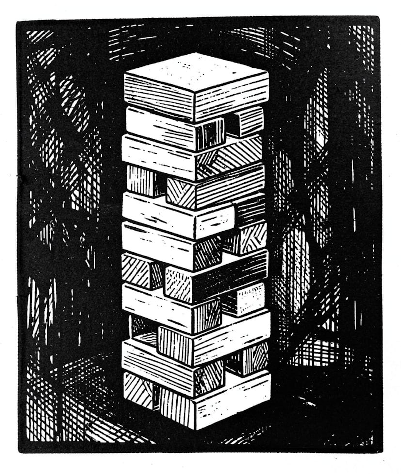
The reclaim work in flight is deliberately minimum-viable in the same spirit as the bump allocator was — pull out the smallest piece the workload demands, leave the tower standing, and don’t add anything that doesn’t pay for itself the moment it lands. The shape:
- Add a per-allocation header carrying size and a one-bit free flag.
- Add an explicit
free(p)p-code instruction that flips the flag and coalesces with adjacent free neighbors. - Maintain a single free list (or a small handful of size classes — still TBD).
- Allocation prefers free-list reuse, falls back to bumping the high-water mark, faults only when both fail.
- No compaction, no GC, no tracing — the OCaml runtime knows when it’s done with a value and is willing to call
freeexplicitly.
That’s still a lot smaller than a real allocator. There’s no defragmentation, no concurrent allocation, no statistics, no debug poisoning, no quarantine. Each of those is a future YAGNI test — if the workload demands it, build it; otherwise leave it out. The new floor is “reclaim works”, not “the allocator is finished.”
The interesting question, once this lands, is whether the OCaml runtime’s allocation pattern is friendly enough to a free-list allocator that fragmentation never bites, or whether some later workload will bite hard enough to force compaction. I genuinely don’t know. That’s fine. The next forcing function will tell me.
Takeaways
- A bump allocator with a no-op
freeis the right call when the workload-set is bounded by demos. It’s fast, small, and impossible to corrupt. - “Real users” expire the assumption. A self-hosted compiler front-end is the smallest realistic workload that requires reclaim, because the working-set is small but the lifetime allocation is unbounded.
- Doubling the heap is a perfectly good response to a memory bug — once. Two doublings is a signal. Three is a confession.
- The next allocator should be exactly as small as the workload demands, and no smaller. Free list, header bit, coalesce on free; defer everything else until something asks for it.
YAGNI didn’t fail here. It cashed out. The allocator was a placeholder all along; today is the day it was supposed to be replaced. The trick was knowing it was a placeholder, and trusting the dogfooding loop to ring the bell when the placeholder ran out.
Future Dogfooding posts will follow the same pattern — a placeholder that earned its keep, the workload that finally outgrew it, and what filling the gap actually looked like. Next up: a postmortem on the reclaim implementation itself, once the OCaml-on-Pascal Tuplet parse can run end-to-end without a heap fault.
Part 1 of the Dogfooding series. View all parts
Comments or questions? SW Lab Discord or YouTube @SoftwareWrighter.
-
1695 words • 9 min read • Abstract
AI Tools #3: sw-checklist --- Reining In AI Coding Agents With a Code-Metrics Ratchet

Why this matters — It is easy to confuse “the AI is fast” with “the AI is producing good code.” Without forcing functions — code metrics, a linter, a TDD loop — a generative agent will happily emit a 600-line file with 12 functions per module and 9 modules per crate, none of which are technically wrong, all of which are technically a mess. The interesting question is not whether to spend on accidental complexity, but which accidental complexity earns its keep.
Resource Link sw-checklist softwarewrighter/sw-checklist No Silver Bullet (Wikipedia) en.wikipedia.org/wiki/No_Silver_Bullet Rich Hickey — Simple Made Easy infoq.com/presentations/Simple-Made-Easy Related Personal Software post pjmai-rs: Navigation History and Fuzzy Completion Comments Discord Brooks: Essential vs Accidental Complexity
Fred Brooks’s No Silver Bullet (1986, later folded into the 20th-anniversary edition of The Mythical Man-Month) draws the line that has framed this argument for forty years:
- Essential complexity is the complexity inherent in the problem itself. Modeling tax law is hard because tax law is hard. There is no clever framework that erases the irregularities of the rules.
- Accidental complexity is the complexity introduced by the tools, languages, and processes we use to attack the problem. CRUD boilerplate, build-system friction, framework idioms — none of it is part of the problem; all of it is part of the cost of solving the problem with the tools at hand.
Brooks’s punchline was that decades of progress had eaten most of the accidental complexity (assemblers, then high-level languages, then garbage collection, then better debuggers), and that future productivity gains would have to come from attacking essential complexity — which is much harder, because it sits inside the problem and refuses to be abstracted away.
That framing still holds. What it does not say — and what is the interesting modern question — is that not all accidental complexity is waste. Some of it is investment. Some of it pays rent.
Hickey: Simple vs Easy, Complect vs Decomplect
Rich Hickey’s Simple Made Easy (Strange Loop 2011) sharpens the same axis from a different angle. Restating it briefly — and this is my paraphrase, not a quote:
- Simple is un-complected: one role, one task, one concept, not braided with anything else. The Latin root is simplex — one fold.
- Easy is familiar and near-at-hand: requires little new learning, fits the muscles you already have.
- Complex is complected — braided, interleaved, two or more concerns sharing a single piece of code.
Hickey’s central claim is that we mistake easy for simple. Reaching for the familiar tool is easy, but it often produces complected code: classes that hold both state and identity, functions that mix decisions with effects, modules that interleave domain logic with transport. Easy now, complex later. Simple, by contrast, is often not easy — it requires more upfront thought to keep concerns separated — but the resulting code is decomplected and stays decomplected as it grows.
Brooks tells you what kind of complexity you are paying. Hickey tells you how the payment compounds. Together they suggest a strategy: accept some accidental cost up front if and only if the payment buys you simple — decomplected, single-role — code.
The Investment Thesis
This is the move I want to defend: some accidental complexity is the cheapest known way to preserve the focus on essential complexity.
A linter is accidental. It rejects code that the language would otherwise compile. The cost is real — the AI agent burns tokens fixing line lengths, the human burns minutes reading diagnostics. The payment is that the next reader can recognize patterns instantly because the surface is uniform.
A TDD loop is accidental. It demands two passes for every line of behavior — the test that fails, then the code that makes it pass. The cost is doubled output. The payment is that essential changes become localized: when the model of the world is wrong, the test names tell you exactly which assumption broke.
Code metrics are accidental. There is nothing wrong, in the language sense, with a 600-line file or a module that holds 12 functions. The payment is that thresholds force the next level of decomposition — a 25-line function ceiling makes you name the sub-step; a 4-functions-per-module warning makes you ask whether two of those functions are really one thing braided with another. Hickey would call that decomplecting.
In all three cases the accidental complexity is paying rent on essential clarity.
sw-checklist as a Forcing Function on AI Agents
sw-checklist is a Rust CLI I run against a project to check conformance. It auto-detects project type — Rust crate, workspace, CLI tool, web UI — and runs the appropriate checks. The interesting checks for this post are the modularity ones:
Check Warn Fail Function lines of code > 25 > 50 File lines of code > 350 > 500 Functions per module > 4 > 7 Modules per crate > 4 > 7 Crates per project > 4 > 7 The numbers themselves are debatable. What is not debatable is what they do to the agent’s behavior over time. There are two regimes:
- Reactive. The agent writes whatever it wants, runs the checklist, sees a failure on “module X has 9 functions,” and rewrites to split. This costs tokens. It also produces good code — the split is often the decomplecting step that the agent would have skipped on its own.
- Anticipatory. Eventually the agent starts splitting before the checklist runs. New code lands closer to the thresholds on the first pass, with named sub-modules and small functions, because the agent has internalized the constraint as a writing style rather than a post-hoc fix-up.
The transition is the interesting moment. It does not happen on day one. It happens after enough cycles that the model has built up a gradient toward the shape of the constraint. From then on, the accidental cost shrinks because the agent is no longer paying for re-writes — it is writing decomplected code on the first try.
The linter and the TDD loop have the same shape. Each one is an accidental cost up front and a style eventually. Each one decomplects a different axis: the linter normalizes the surface, TDD localizes the model, sw-checklist enforces the decomposition.
The Ratchet

Tech debt grows when anything is allowed to slide. The naive policy — “we’ll clean it up later” — reliably produces a heap. The opposite policy — “no debt, ever” — reliably produces paralysis.
The policy I aim for is a ratchet:
- The wrench turns one way.
- Sometimes a tooth slips back — a temporary hack, a function over the threshold, a test marked
ignorewhile a bigger refactor lands. - The next click must be forward. Slips are bounded; the trend is monotone.
A ratchet does not promise that every commit reduces debt. It promises that the cumulative direction is reduction. That promise is enforceable: at every cycle, ask “is the metric better or worse than last commit?” and refuse to merge a regression unless it is consciously, visibly, paying for a larger forward turn.
This is the connecting tissue between the Brooks framing and the day-to-day. If accidental complexity is investment, the ratchet is what protects the investment from being clawed back by the next sprint’s deadline.
De-complexifying as a Practice
Pull the threads together:
- Brooks: distinguish accidental from essential complexity, and spend on accidental cost only where it preserves essential clarity.
- Hickey: aim for simple (decomplected), not just easy (familiar). The two are not the same and confusing them is how complected code grows.
- The investment thesis: linter, TDD, and code metrics are accidental costs that pay rent in decomplecting — they make essential complexity stay visible.
- The forcing function: AI agents respond to constraints first reactively, then anticipatorily. The sooner the constraint is in the loop, the sooner the agent’s output moves from messy-and-correct to focused-and-correct.
- The ratchet: tech debt may slip a tooth but the wrench only turns one way. Cumulative direction matters more than per-commit purity.
The phrase I keep coming back to is de-complexify. It is not the same as simplify. Simplifying is reducing scope; de-complexifying is keeping the same scope while pulling the strands apart so each strand has one job. Hickey’s word for the move is decomplect. Brooks would call the result a code base where the essential complexity is visible and the accidental complexity is bounded.
Vibe-coding done well is exactly that: AI agents producing focused, decomplected code, fast, because the constraints are doing the de-complexifying work in the background and the agent has learned to write inside them.
The constraints cost something. They are accidental complexity. They are also the only way I have found to keep the essential complexity in view long enough to actually solve it. sw-checklist is one piece of that personal-software toolkit — a small CLI whose only job is to make the next decomplecting step impossible to ignore.
Part 3 of the AI Tools series. View all parts | Next: Part 4 →
Comments or questions? SW Lab Discord or YouTube @SoftwareWrighter.
-
2481 words • 13 min read • Abstract
Saw #8: Tuplet, Smalltalk-on-BASIC, Forth-from-Forth, sw-MLPL Split, and I2C on COR24

Why Sharpen the Saw? — The name comes from Covey’s Habit 7: stop cutting long enough to sharpen the blade. This series tracks weekly investment in the tools themselves—agent orchestration, testing infrastructure, compiler toolchains, language platforms—so the feature work on top goes faster.
Resource Link Tuplet github.com/sw-vibe-coding/tuplet Smalltalk on COR24 BASIC github.com/sw-embed/sw-cor24-smalltalk Smalltalk video (YouTube Short) youtube.com/shorts/fL5NLSKkLoU Forth-from-Forth (proto-forth-wasm) github.com/sw-vibe-coding/sw-fth-wasm — live demo COR24 Demo Hub (Status tab) sw-embed.github.io/web-sw-cor24-demos Repos & Live Demos Table below Prior Post Saw #7: Prolog, Many-Agent Isolation, Self-Hosting Assembler, and MLPL Comments Discord Tuplet: A Glyph-and-Whitespace Language Playground
Tuplet is a new experimental infix language with first-class named tuple bundles, multi-output verbs, call-site argument splicing, and a glyph-heavy surface syntax. The kernel is small (~10 forms); everything else—
if/then/else,while, every operator, every helper—is defined in a prelude using a single mechanism called mint (▪, BLACK SMALL SQUARE, U+25AA). User code can read, replace, or extend the same definitions the prelude uses. Tuplet compiles to Forth and runs on the COR24 runtime.A taste of the surface syntax—a
Powerverb that uses Tuplet glyphs for type signature, assignment, and a piecewise definition:⎧ 1 → ▪ Power (n : ℤ e : ℤ) → (p : ℤ) ← ⎨ loop e times iff e is positive ⎩ n (×) →The glyphs in that fragment are: ▪ (BLACK SMALL SQUARE, U+25AA, mint), ℤ (DOUBLE-STRUCK Z, U+2124, integer type), → (RIGHTWARDS ARROW, U+2192, map / signature), ← (LEFTWARDS ARROW, U+2190, assign), ⎧⎨⎩ (LEFT CURLY BRACKET UPPER HOOK + MIDDLE PIECE + LOWER HOOK, U+23A7/U+23A8/U+23A9, multi-line piecewise group), and × (MULTIPLICATION SIGN, U+00D7, multiplication). Every glyph has an ASCII fallback the lexer accepts, and the lexer folds Unicode forms to ASCII canonicals at lex time so AST output and error messages stay portable. See
docs/glyphs.mdfor the full alphabet.Two things make Tuplet immediately practical:
- Implementation language: Tuplet’s host implementation is an OCaml subset that runs on sw-cor24-ocaml. Using OCaml as a load-bearing part of the toolchain forced a round of new features in the OCaml interpreter—details in the Smalltalk-and-Tuplet section below.
- Compilation target: Tuplet lowers to Forth, so it inherits whatever the COR24 Forth and Forth-from-Forth efforts deliver. New Forth features cascade into Tuplet for free.
Glyph Input Infrastructure: Espanso and Emacs
A glyph language is unusable if you can’t type it. The glyph-entry layer is its own piece of the toolchain, and it now has two parts:
- Espanso is a cross-platform text expander. Installing and configuring Espanso gives every editor and terminal a shared way to type Tuplet glyphs by short trigger sequences. The same configuration also covers GNU APL glyph entry—APL has the canonical “language with non-ASCII glyphs” problem, and Espanso solves both at once. See
docs/cli-inputs.mdfor the Tuplet trigger conventions. - Emacs has its own glyph-entry configuration so the same triggers work natively in Emacs buffers without going through Espanso. TeX-style input methods, Agda-style mappings, and a custom Quail input method are all options—see
docs/emacs-inputs.md. This keeps the editing experience consistent whether you’re in a terminal REPL, a browser-based demo, or an Emacs buffer.
Glyph entry counts as Sharpen the Saw work because it is infrastructure for future experiments: every new language that wants non-ASCII syntax—Tuplet, GNU APL, the next experiment—rides on the same input layer.
Smalltalk on COR24 BASIC: Dogfooding as a Forcing Function

A small integer/toy Smalltalk is now running, implemented in COR24 BASIC v1—a 26-variable, no-array, integer-only BASIC interpreter. The Smalltalk is in the spirit of the ~1000-line BASIC-hosted Smalltalk evaluator that Alan Kay’s group built in 1972. It has a tagged-pointer object encoding (low-bit-1 SmallIntegers, low-bit-0 heap pointers), 14 bytecodes, 6 primitives in v0, and a real
CLASSOF -> LOOKUP -> ACTIVATE -> primitive-or-frame-pushdispatch loop. The whole heap, method table, and frames live in 1024 24-bit words ofPEEK/POKEscratch RAM. Three nested fetch/decode/execute loops (p-code VM, BASIC interpreter, Tinytalk VM) run at all times.Video walkthrough (YouTube Short): https://www.youtube.com/shorts/fL5NLSKkLoU
The point is not speed. The point is to make the OO mental model visible—every dispatch step is a numbered BASIC line you can single-step through—and to dogfood COR24 BASIC by writing a real, recognizable system in it. The forcing function worked: writing Smalltalk in BASIC immediately revealed gaps. Six BASIC feature requests landed and closed this week:

BASIC issue Feature FR-1 DIM integer arrays FR-2 DATA / READ / RESTORE statements FR-3 ON expr GOTO/GOSUB statements FR-4 MOD operator FR-5 Bitwise operators (BAND/BOR/BXOR/SHL/SHR) FR-6 CONT after STOP Tagged-pointer dispatch needs the bitwise ops; method tables and bytecode arrays want
DIM;DATA/READis the natural way to ship the boot image;ON expr GOTOis the dispatch-jump that powers the bytecode interpreter. Each was a real shortcoming Smalltalk hit, not a speculative wishlist item. The BASIC live demo ships them all.The same forcing-function pattern played out for Tuplet on the OCaml side. Eleven OCaml interpreter issues closed in the last 24 hours, almost all driven by Tuplet’s host code:

OCaml issue Feature #1 TRAP 2 in demo_adventure(round-trip bug)#2 User-defined variant types (algebraic data types) #3 Top-level letbindings (withoutin EXPR)#4 String escapes ( \n,\t, …) and arbitrary tuples (3+)#5 Multi-line matchexpressions#6 Mutable references ( ref,!,:=)#7 Record types and field access #8 List combinators ( List.map,List.fold_left,List.filter)#9 Block comments (* ... *)#10 Char literals 'a'+Char.code/Char.chr#11 Exceptions ( raise/try/with) or aResulttypeA lexer, AST, and IR lowering pipeline needs records, variants, top-level lets, multi-line match, mutable refs, and exceptions just to be writable. The OCaml live demo now ships every one of those. The Forth side picked up the matching upgrades—
:NONAMEfor anonymous colon definitions and aSEE-CFAtruncation fix—in sw-cor24-forth over the same window.Forth-from-Forth: A Browser-Native Forth via WASM
Forth-from-Forth (
proto-forth-wasm) is a browser-native Forth running on Rust/WASM. The RustMachineowns the data stack, return stack, memory, dictionary, tokenizer, compiler, and VM loop; colon definitions compile to an opcode IR; user-word execution runs on an iterative VM loop with no host-stack recursion for nested calls. The vocabulary already covers arithmetic, stack shuffling, comparisons, structured control flow (IF/ELSE/THEN,BEGIN/UNTIL,BEGIN/WHILE/REPEAT,DO/LOOPwithI), memory (VARIABLE,CONSTANT,@,!,+!,ALLOT), the return stack, I/O, and introspection (SEE,WORDS).The live demo puts the REPL, source pane, stack, dictionary, output, history, and trace all on one page. WASM matters here for the same reason a self-hosting toolchain matters elsewhere: zero-install distribution. A reader can land on the page and have a working Forth in seconds.
Two Forth-in-Forth issues closed this week pulled the project closer to self-hosting at the language level: #1 added a hashed dictionary to speed up
FIND, and #2 addedDO/LOOP,?DO,WHILE/REPEAT,AGAIN,CONSTANT, andVARIABLEto the Forth-in-Forth implementation. Open issue #3 tracks the remaining standard words:+LOOP/J/LEAVE,DOES>,RECURSE,PICK/ROLL/?DUP/MIN/MAX/<=/>=/<>.A Forth-builder is in planning—a small kit (inner interpreter, dictionary, I/O backend, target word set) that composes Forth systems by configuration instead of by fork. Once the builder exists, spinning up a new Forth flavor for an experiment becomes a build-time decision.
sw-MLPL: 35 GB Forces a Split into Parallelizable Pieces

sw-MLPL (live demo) hit a different kind of forcing function this week: its build directory blew past 35 GB on a MacBook, and that is without the CUDA backend wired in yet. A single repo trying to hold a CPU runtime, the MLX backend, a future CUDA backend, an interpreter, a compiler, a REPL, and a Web UI is not a structure that fits on one laptop.
The fix is to split:
- Linux/CUDA only — one fork that targets NVIDIA CUDA and lives on a host with the disk space and toolchain to support it.
- Mac/MLX only — a sibling fork that stays on Apple Silicon and the MLX unified-memory path, where the build stays small enough to iterate on a laptop.
- Web UI separated — the in-browser demo carved out into its own repo, decoupled from the runtime build cycle.
- Compiler and REPL separated — the two have different dependency profiles and different test harnesses; separating them lets each grow without dragging the other’s build along.
The win is not just disk space. Once the project is split, different hosts can develop different pieces in parallel: a Linux/CUDA box pushes the GPU backend while a MacBook iterates on MLX or the compiler, and neither waits on the other’s artifacts. The Web UI repo’s CI doesn’t care which backend any given commit targets. This is the same pattern the COR24 stack uses by default—small, single-purpose, parallelizable repos—applied retroactively to a project that grew past the point of fitting in one place.
I2C on the COR24 Emulator

The COR24 emulator is gaining I2C support, with example programs to drive it. I2C unlocks the obvious next layer of peripheral experiments—temperature/pressure sensors (the BMP280 repo is already in the tree), small EEPROMs, OLED displays, and any of the usual hobbyist breakout boards. I2C is the right first bus for the emulator: low pin count, well-documented protocol, plenty of devices to talk to, and the bring-up code is small enough that the Smalltalk and Tuplet languages above could plausibly drive a real sensor in a future demo.
The pattern is the same as everywhere else in this post: build the platform piece (the bus, the examples) so that future feature work has somewhere to land.
Demo Site: Status Tab Tracks the New Languages
The COR24 demo hub now has a Status tab that tracks the languages, their recent commits, and their open issues in one place. Adding Tuplet and Smalltalk to the lineup made the per-language pages harder to skim, so the Status tab consolidates:
- The current language list (now including Tuplet and Smalltalk, alongside PL/SW, SNOBOL4, MLPL, BASIC, Forth, OCaml, Pascal, APL, MacroLisp, P-code, TinyC, and the assemblers).
- Recent commits per language—a single cross-repo activity feed.
- Open issues per language, so the in-flight work is visible without bouncing between GitHub repos.
Demo Hub (and Status tab): sw-embed.github.io/web-sw-cor24-demos/#/
The Status tab is the same kind of investment as the glyph-input layer and the I2C bus: infrastructure for moving faster, not a feature in any one language. New languages plug into it; the cost of adding the next one is now bounded.
Repos and Live Demos
Project GitHub Live Demo Tuplet sw-vibe-coding/tuplet in development Smalltalk on COR24 BASIC sw-embed/sw-cor24-smalltalk sw-embed.github.io/web-sw-cor24-smalltalk Forth-from-Forth (WASM) sw-vibe-coding/sw-fth-wasm sw-vibe-coding.github.io/sw-fth-wasm COR24 BASIC sw-embed/sw-cor24-basic sw-embed.github.io/web-sw-cor24-basic COR24 Forth sw-embed/sw-cor24-forth sw-embed.github.io/web-sw-cor24-forth COR24 OCaml sw-embed/sw-cor24-ocaml sw-embed.github.io/web-sw-cor24-ocaml COR24 Emulator (I2C) sw-embed/sw-cor24-emulator sw-embed.github.io/cor24-rs sw-MLPL sw-ml-study/sw-mlpl sw-ml-study.github.io/sw-mlpl COR24 Demo Hub sw-embed/web-sw-cor24-demos Demo Hub What’s Next
Tuplet: Get the Tuplet live demo working alongside the other COR24 language demos, and add a way to enter glyphs directly in the Tuplet web UI (so visitors don’t need Espanso or Emacs configured locally to try the demo).
Smalltalk on COR24 BASIC: Get the Smalltalk live demo working—a browser-hosted version of the BASIC interpreter running the Tinytalk image, so the YouTube walkthrough has a hands-on counterpart.
Glyph Input + Emacs: Publish concrete Emacs configuration examples (init snippets, Quail rules, TeX-style mappings) drawn from
docs/emacs-inputs.md, and add org-mode support—which means babel blocks for Tuplet and every other COR24 language (BASIC, Forth, OCaml, PL/SW, SNOBOL4, etc.). Babel-blocks across the language set turns org-mode into a real notebook for the COR24 stack.Forth-from-Forth: Close the remaining standard Forth words (sw-cor24-forth #3) and start the Forth-builder kit so new Forth flavors compose by configuration.
sw-MLPL Split: Land the four-way split (Linux/CUDA, Mac/MLX, Web UI, separated Compiler vs. REPL) and confirm each piece builds cleanly on a host that doesn’t have the others’ dependencies. Republish the live demo from the new Web UI repo.
COR24 Emulator I2C: Land the first round of I2C example programs end to end (sensor reads, EEPROM round-trip), then expose I2C from the higher-level languages so a Tuplet or Smalltalk program can drive a peripheral.
Forcing functions sharpen languages faster than feature lists do. Follow for more Sharpen the Saw updates.
Part 8 of the Sharpen the Saw Sundays series. View all parts | Next: Part 9 →
Comments or questions? SW Lab Discord or YouTube @SoftwareWrighter.
-
1278 words • 7 min read • Abstract
Rabbit-hole #5: FORTH --- Retargetable Codegen and the Forward-Reference Problem

Resource Link Play in Browser COR24 Forth Demo Kernel Repo sw-embed/sw-cor24-forth Prior post Rabbit-hole #4: FORTH — Dictionary Compaction and Specialized Images Overview post Embedded #3: Self-Hosting Spectrum Comments Discord The Vertical Split Was Only Half the Problem
Part 4 framed the Forth composer as a way to build different profiles from the same source:
Profile Keeps Drops dev names, FIND,CREATE, REPL, instrumentationalmost nothing runtime compiled CFAs, primitives, inner loop names, compiler, REPL, dead words debug-runtime compiled CFAs plus symbols and trace hooks full interactive machinery That is vertical specialization. The target machine stays the same; the amount of Forth you carry into the final artifact changes.
Retargetable codegen asks a different question:
What if the profile is the same, but the output machine changes?
COR24 wants one shape of branch. WASM wants another. RV32I has registers and load/store rules that do not resemble a tiny threaded-code VM. S/360 brings condition codes, base registers, and a whole cultural memory of what “assembly” means.
If the compiler is self-hosted, this cannot be solved by hiding everything behind a giant external backend forever. Eventually the Forth system itself needs to describe what it emits.
The Tempting Bad Design
The easiest design to imagine is also the one that rots first:
: EMIT-CALL
  TARGET-COR24 IF ... THEN
  TARGET-WASM  IF ... THEN
  TARGET-RV32I IF ... THEN
  TARGET-S360  IF ... THEN ;
Do that for
CALL,BRANCH, literals, stack effects, memory access, returns, labels, and relocations, and the compiler becomes a pile of target checks. Every new target edits shared code. Every feature test is now a backend integration test. The source language has no clean boundary from the machines it targets.That is not a retargetable compiler. That is a compiler with a target-shaped rash.
A Better Boundary: Operations, Not Instructions
The useful split is between semantic operations and target encodings.
The front half of the Forth compiler should talk in operations:
Operation Meaning op-call wordtransfer to a known word and return op-lit valueplace a literal on the data stack op-branch labelunconditional control flow op-0branch labelbranch if top of stack is false op-load addrfetch from memory op-store addrstore to memory op-exitreturn from colon definition The backend owns how those operations become bytes, cells, threaded CFAs, WASM instructions, or assembly text.
That boundary is what lets COR24 stay simple while a future WASM target does something entirely different.
The Forward-Reference Problem
Forth normally likes definitions to appear before use. A simple single-pass compiler can get very far with that rule:
: SQUARE DUP * ; : AREA SQUARE * ;AREAcan callSQUAREbecauseSQUAREalready exists.But real systems eventually want cycles:
: EVEN? DUP 0= IF DROP TRUE EXIT THEN 1- ODD? ;
: ODD?  DUP 0= IF DROP FALSE EXIT THEN 1- EVEN? ;
At the moment
EVEN?is compiled,ODD?does not exist yet. A name lookup cannot produce a CFA because there is no CFA to find.There are three classic ways out:
Strategy Tradeoff Require ordering simple compiler, awkward programs Add declarations more syntax, better compile-time knowledge Emit unresolved references needs fixups, enables natural structure For a self-hosting Forth that wants retargetable codegen, unresolved references are the interesting path. They turn the compiler into a small linker.
Fixups Are the Linker Hiding in the Compiler

When the compiler sees a reference to a word it cannot resolve yet, it can emit a placeholder and record a fixup:
Field Example unresolved name ODD?use site byte/cell offset inside EVEN?relocation kind call target, branch target, literal address target profile dev, runtime, debug-runtime backend COR24, WASM, RV32I, S/360 Later, when
ODD?is defined, the linker pass patches every recorded use site.This is not only for mutually recursive colon definitions. The same mechanism handles branch labels, separately compiled modules, runtime-image compaction, and target backends whose branch instruction cannot be encoded until the distance is known.
Why This Belongs With the Composer
Part 4’s composer decided which words survive into an image.
Part 5’s composer has to decide where surviving words land, what unresolved references point to, and how target-specific relocation works.
That suggests one pipeline:
- Parse and compile source into target-neutral operations.
- Record unresolved words and labels as fixups.
- Resolve names after each module or full source load.
- Choose a profile: dev, runtime, debug-runtime.
- Compact the dictionary for that profile.
- Hand surviving operations and fixups to the target backend.
- Emit the final artifact and a manifest of what was resolved.
The same manifest that makes dictionary compaction auditable also makes retargeting auditable. If a runtime image drops a word that a backend still needs, the build should fail with a name and a fixup site, not a mystery crash.
Target Notes
This section needs measurements and examples from actual backend sketches.
COR24
COR24 is the baseline: small, explicit, close to the current Forth image model.
Notes to fill in:
- direct-threaded vs subroutine-threaded options
- branch range and call encoding
- how much relocation state is needed for compacted runtime images
WASM
WASM is structured, typed, and not just “assembly with different mnemonics.”
Notes to fill in:
- structured control flow vs arbitrary branch labels
- stack machine overlap with Forth’s data stack
- imports/exports for host integration
RV32I
RV32I is useful because it forces the compiler to be honest about registers and memory.
Notes to fill in:
- stack pointer conventions
- immediate range limits
- call/return sequence
S/360
S/360 is useful because it makes relocation and base registers visible.
Notes to fill in:
- base register setup
- literal pools
- condition code mapping
What Comes Next
The next rabbit-hole after this one should probably stop talking about compiler structure and show an actual thin backend: take one tiny Forth source file, emit two target artifacts, and compare the fixup manifests side by side.
The composer idea only matters if it survives contact with a second target.
Part 5 of the Down the Rabbit-Hole series. View all parts
Comments or questions? SW Lab Discord or YouTube @SoftwareWrighter.
-
2066 words • 11 min read • Abstract
Rabbit-hole #4: FORTH --- Dictionary Compaction and Specialized Images

Resource Link Play in Browser COR24 Forth Demo Kernel Repo sw-embed/sw-cor24-forth Prior post Rabbit-hole #3: FORTH — Life After Hashing Overview post Embedded #3: Self-Hosting Spectrum Comments Discord Two Different Forths, Same Source
A working Forth environment does a lot of things at once:
- Reads source text, tokenizes, looks up names → interpret/compile
- Holds a live dictionary, walked by
FIND, grown byCREATE - Exposes a REPL for interactive use
- Runs user-level compiled code (the actual work)
- Sometimes: profiles, instruments, debugs
In a development Forth, all of this matters. You’re compiling new words, reloading
.fthfiles, poking at things via.SandWORDS. The dictionary must be searchable by name, CREATE must work, the REPL must respond.In a deployed Forth — the kind you’d flash onto an FPGA or ship in a firmware image — most of that is overhead. The deployed program already exists as compiled bytecode. It doesn’t need FIND. It doesn’t need CREATE. It doesn’t need the REPL. It doesn’t even need the names of the words it calls, because the calls are already resolved.
Dictionary compaction is the name for the gap between those two Forths. Specialized-image building is how you cross it.
Three Optimization Layers
Posts 2 and 3 sat entirely in layer 1. This post introduces layers 2 and 3.
Layer Target Examples 1. Dev-time lookup Make FIND fast in the dev image Numeric fast path · recent-hit cache · hot-token cache (Part 3) 2. Dictionary compaction Shrink what gets shipped Drop shadowed words · strip instrumentation · remove dead code 3. Whole-app specialization Eliminate the interpreter for production Drop FIND · drop CREATE · drop REPL · ship only compiled CFAs Each layer is opt-in. Each is a different build artifact produced from the same source tree. A composer sits at the top and chooses which layers to apply for a given target profile.
A Forth Composer
The mental shift, once you’ve done this a few times:
You’re not building “a Forth.” You’re building a Forth system generator that can assemble different Forth flavors for different use cases.
Named profiles for common builds:
Profile Lookup subsystem Instrumentation Image Good for simpleLinear walk only Off Full dev dict Teaching, debugging instrumentedLinear + recent cache + counters On Full dev dict Profiling real workloads optimizingLinear + both caches On, driving reorder Compacted dev dict Interactive, fast boot runtimeNone (no FIND) Off Compiled CFAs only Deployed app debug-runtimeNone Minimal ( assert,trace)Compiled CFAs + symbols Crash-reproducible deploy The core is the same in every profile: stacks, threading, primitives, inner loop. Everything above that is a composition of optional modules and policies. The composer’s job is to know which modules are required, which conflict, and how to wire them together for the requested profile.
This is cleaner than “one Forth tries to be everything.” It matches the spirit of the self-hosting spectrum post’s phased migration: different axes are orthogonal, so treat them that way.
What Compaction Actually Removes
For profile
runtime(the most aggressive), the compactor walks the live dictionary and drops:Shadowed redefinitions. Forth lets you redefine a word. The old definition stays in the dictionary, unreachable by name (FIND walks newest-to-oldest, hits the new one first) but still taking space. In a runtime image, shadowed entries are pure dead weight. Drop them.
Bootstrap-only words. Words that exist only to load the source. Things like
,DOCOL,CONSTANT,VARIABLE,CREATE,:,;,IMMEDIATE. If the runtime image doesn’t compile new words at runtime, none of these are needed — they were scaffolding used during loading.Interpreter loop.
INTERPRET,QUIT,WORD,FIND,NUMBER. A runtime image that runs one entry point (MAINor whatever) doesn’t read text, doesn’t tokenize, doesn’t look things up. The whole outer loop is gone.Instrumentation. Any counters, profiling hooks, trace points. These were for building the optimized image; they don’t go into the deliverable.
Developer-only helpers.
.S,DUMP,WORDS,SEE,DEPTH, diagnostic decorations. Useful at the REPL; useless in deployment.Name strings. The aggressive move: drop the name field on every dictionary entry. Runtime callers reach words by CFA, not by name, so the strings are only readable by a human via
SEEandWORDS— both dropped in the previous step. 40-char headers become 4-char (flags byte + link + CFA).What’s left after all that: the data stack, the return stack, a handful of primitives still needed by compiled code (
+,@,!,DUP, etc.), the inner loop (NEXT), and the compiled CFAs of words the application actually calls. On COR24, that’s the difference between a ~3KB dev image and a ~600-byte runtime image.The Real Implementation Burden: Pointers

Removing words is the easy part. Rewriting all references to those words is where dictionary compaction earns its reputation.
Every compiled colon definition is a sequence of CFA pointers:
SQUARE: DOCOL | <DUP's CFA> | <*'s CFA> | EXITIf the compactor removes a shadowed
*and the remaining*lives at a different address, every single compiled definition that points at the old*now points at a stale address. You have to find them all and rewrite them.That requires:
- An authoritative record of which word each CFA originally named. Names are dropped in the final image but must exist during compaction.
- A walk of every compiled body, looking at each cell, asking “is this a CFA pointer?” and if so “which word does it refer to now?” and rewriting accordingly.
- Fixups for literal addresses (from
LIT), branch targets (fromBRANCH/0BRANCH), and any word-to-word references stored in data cells. - A reproducible layout algorithm so two runs over the same source produce the same image. This matters for CI.
Under the hood, this is the same relocation problem a linker solves. The Forth composer is a linker for Forth objects. It just happens to be written in Forth.
Two techniques help:
- Build a new image rather than editing the old one. Start from a clean allocation, stream surviving words through one-by-one, fix up pointers as you go. This is much easier than trying to edit-in-place and much easier to test.
- Do not reorder words until all compaction is done. The pointer-rewrite pass is simpler when you know the old → new CFA mapping is stable. Reordering for cache locality, if you do it, is a separate pass over the already-compacted image.
Profile-Driven Optimization
Compaction without data is guesswork. What goes, what stays, what gets reordered — the composer needs a profile that captures real usage.
The right counters to capture during a profiling run:
Counter What it measures Drives source-interpret-countTimes word looked up at REPL Recent cache tuning source-compile-countTimes word looked up during source loading Hot cache seeding runtime-execute-countTimes compiled CFA executed Dictionary reordering · inlining last-used-passWhich build step last referenced word Shadowed / dead-code detection The PROFILE-ON / PROFILE-OFF mental model from the composer:
PROFILE-ON
( load source, run demo workload, exercise edge cases )
PROFILE-OFF
DUMP-COUNTS   \ writes the profile to an external file
BUILD-OPT-IMAGE use-profile=demo.prof target=runtime
Counts are written external to the dictionary so the composer can re-use them across builds and compare policies. The same profile data can drive multiple output images (a runtime target + an instrumented dev target) without recollecting measurements.
The Overfitting Trap
Optimizing against a demo corpus is seductive, and it’s wrong in the same ways micro-benchmark tuning is wrong.
If the profile comes from 25 example
.fthfiles and those are the only workloads the deployed image will ever see: perfect, overfit freely. The deployed image is a fixed-function artifact; fitting it to its workload is the whole job.If the deployed image will see workload
#26that looks different: compaction that was fine against the 25 can silently drop words that#26needs, or reorder the dictionary in ways that make#26slow. The composer can’t catch this unless#26is in the profile.Mitigations:
- Keep a canary
.fthfull of standard Forth idioms that the compacted image must still run. Regression-check it on every build. - Have at least one “safe” profile that retains more than you strictly need, for deployments whose workload is uncertain.
- Be explicit about what got cut. The compactor should emit a manifest of which words it dropped, which it kept, and why. Surprises in deployment trace back to surprises in that manifest.
The classic advice: optimize the workload you have, guard against the workload you don’t. The composer makes both easier — different profiles for different risk tolerances — but it doesn’t automate the judgment call.
Where This Lands
Three layers of optimization, one composer selecting profiles. The runtime profile ships a Forth that doesn’t look much like Forth: no REPL, no interpreter, no dictionary-by-name. Just compiled CFAs and a tiny inner loop. Some people call this “a runtime,” not a Forth. Either framing is fine. The point is that the same source produces both the interactive dev Forth and the minimal runtime deliverable — by composition, not by a separate rewrite.
The phase-4
forth-from-forth/work naturally wants this framing. A Forth-hosted cross-compiler already has to reason about “which words end up in the output image.” Making that reasoning explicit — the composer decides — turns an implicit dependency tree into an explicit build pipeline.What’s Next
Compaction collapses vertically — strip unused words, drop unused features. The next rabbit-hole post asks about horizontal compaction: when the same Forth source has to target different ISAs (COR24, WASM, RV32I, S/360), how do you partition the compiler so only the backend changes? And what happens when the compiler has to reference words that don’t yet exist — the forward-reference / mutual-recursion problem that every self-hosted compiler eventually faces.
That’s Rabbit-hole #5: FORTH — Retargetable Codegen and the Forward-Reference Problem.
One source, many artifacts. The Forth composer is just the recognition that different deployments want different Forths — and the discipline to stop pretending otherwise.
Part 4 of the Down the Rabbit-Hole series. View all parts | Next: Part 5 →
Comments or questions? SW Lab Discord or YouTube @SoftwareWrighter.
-
1951 words • 10 min read • Abstract
Rabbit-hole #3: FORTH --- Life After Hashing

Resource Link Play in Browser COR24 Forth Demo Kernel Repo sw-embed/sw-cor24-forth Prior post Rabbit-hole #2: FORTH — FIND and the Cost of a Name Overview post Embedded #3: Self-Hosting Spectrum Comments Discord The Post-Hash Toolbox
Three optimizations, all cheaper than a hash, all written in pure Forth. None of them require a side table, none require touching dictionary headers, none require boot-time setup. Each one trades a little code for a better hit rate on the patterns that actually show up in source files.
Optimization Cost Hit pattern Numeric fast path ~5 lines of Forth Any token starting with a digit or -<digit>Recent-hit cache (N entries) ~10 lines + N × 2 cells of memory Tokens repeated within a short window Hot-token cache (top-K) ~20 lines + K × 2 cells + some accounting The handful of names that appear 100s of times They’re orthogonal. You can ship any one, any two, or all three. The order below is the order I’d install them in: each next one is a little more work for a little more payoff.
Optimization 1: Numeric Fast Path
Every
.fthsource file has numbers in it. In the all-asm INTERPRET, each number makes FIND walk the dictionary, fail to find a match, and then fall through to NUMBER. That’s wasted work — you can tell by the first character that no dictionary word will match.The fix is a one-line pre-check at the top of INTERPRET:
: INTERPRET
    WORD DUP C@                   \ token (addr len) first-char
    [CHAR] 0 [CHAR] 9 WITHIN
    IF  NUMBER  EXIT  THEN        \ starts with a digit — skip FIND
    ... (normal FIND path) ...
;
(Handle
-<digit>with one more check. Handle$or0xhex prefix if your Forth takes those.)On a
.fthsource file likeexamples/fib.fth:: FIB ( n -- n' ) DUP 2 < IF EXIT THEN DUP 1- RECURSE SWAP 2- RECURSE + ;The tokens
2,1-,2-all start with digits (well,1-and2-look like numbers until the dash is consumed and the remaining part doesn’t parse — some Forths special-case1-as a word anyway; take the simple path and let FIND confirm after the numeric parse fails). The main point: literal numbers like2get a direct routing to NUMBER and skip FIND entirely.Measurement shape. On the COR24 core loading
examples/*.fth, numeric tokens are ~20% of the input stream. Fast-pathing them avoids the equivalent fraction of dictionary walks. One branch, huge payoff.Caveat. If your Forth lets words start with digits (
2dup,2drop,4th), the fast path has to fall back to FIND on “might-be-a-word” failures. In practice that means: try NUMBER first, and if NUMBER rejects the whole token, then FIND it. The rejection is fast — NUMBER aborts on the first non-digit.Optimization 2: Recent-Hit Cache
The circular-buffer design. Keep the last N successful
(hash, cfa, flags)tuples — call it 8 or 16 entries. Every FIND first probes the circular buffer by hash; on hit, return immediately. On miss, walk the dictionary, then insert the result into the next slot of the buffer (overwriting the oldest).Rough structure in Forth:
16 CONSTANT RECENT-SIZE
CREATE recent-hash  RECENT-SIZE CELLS ALLOT
CREATE recent-cfa   RECENT-SIZE CELLS ALLOT
CREATE recent-flags RECENT-SIZE CELLS ALLOT
VARIABLE recent-next   \ index where the next insert lands

: recent-lookup ( h -- cfa flags | 0 0 )
    RECENT-SIZE 0 DO
        DUP recent-hash I CELLS + @ =
        IF  DROP
            recent-cfa   I CELLS + @
            recent-flags I CELLS + @
            UNLOOP EXIT
        THEN
    LOOP  DROP 0 0 ;

: recent-insert ( h cfa flags -- )
    recent-next @  >R
    R@ recent-flags + !
    R@ recent-cfa   + !
    R@ recent-hash  + !
    recent-next @ 1+  RECENT-SIZE MOD  recent-next ! ;
A FIND now becomes:
: FIND  ( addr len -- cfa flags )
    hash-name recent-lookup  ?DUP IF EXIT THEN  DROP
    dict-walk  ( returns cfa flags or 0 0 )
    DUP IF  \ found — remember it
        2DUP hash-name -ROT recent-insert
    THEN ;
Where
hash-nameis a cheap hash (just XOR the first 3 characters, for example) — the full XMX is overkill here because we only need to distinguish N=16 candidates, not partition 256 buckets.Why it works. Temporal locality. In a typical
.fthblock:: SQUARE DUP * ; : CUBE DUP SQUARE * ; : FOURTH SQUARE SQUARE ;DUP,*,SQUARE, and;each get looked up multiple times within a few-token window. The recent-hit buffer catches all of it. Buffer size N=8 is enough for most Forth source; N=16 is generous.Cost.
N × 3 cells ≈ 72 bytesfor a 16-entry cache on COR24 (3-byte cells). Linear scan of 16 entries is ~48 COR24 instructions worst case, fewer on hit. Compare to a hash-table miss walking a chain of 15 — the circular buffer wins whenever the hit rate is above ~25%.Optimization 3: Hot-Token Cache
The recent-hit cache catches local repetition. What it misses: tokens that appear in many different contexts —
DUP,!,@,IF,;. These words show up hundreds of times across a full core-loading pass, but rarely in back-to-back tokens. The recent buffer evicts them between hits.The hot-token cache handles that shape. Top-K by frequency. K is small — 4 or 8 entries is plenty — because Forth’s name distribution is severely top-heavy: the top 10 words typically account for 40–60% of all lookups in a core.
Structure is essentially the recent cache plus frequency counters:
8 CONSTANT HOT-SIZE
CREATE hot-hash  HOT-SIZE CELLS ALLOT
CREATE hot-cfa   HOT-SIZE CELLS ALLOT
CREATE hot-flags HOT-SIZE CELLS ALLOT
CREATE hot-count HOT-SIZE CELLS ALLOT
On every dictionary walk that finds a word:
- Increment the count for that word’s bucket.
- If any bucket’s count exceeds the minimum in the top-K, promote the new entry and evict the former minimum.
Lookup probes the hot cache first, then the recent cache, then does the dictionary walk.
Why it works. Forth’s word-frequency distribution is Zipf-like. The top 8 names cover roughly half of all lookups in a typical
.fthcorpus; the top 32 cover nearly all of them. A tiny K-wide cache pins the most-frequent names in place regardless of temporal locality.Pitfall. If you promote aggressively on every increment, the top-K churns on early workloads before settling. Add a small hysteresis (only promote when the count exceeds the minimum by some margin), or seed the cache after a profiling pass has accumulated stable counts.
The Instrumentation Question
You can’t build the hot-token cache honestly without counting. And the counter has to count the right thing.
There are three plausible counts, and they’re not the same:
Counter What it measures Useful for Source-interpret count How often a name is looked up while reading .fthsource in interpret modeTuning the recent cache for REPL use Source-compile count How often a name is looked up while reading .fthsource in compile modeTuning the recent/hot cache for .fthloadingRuntime execution count How often a compiled word runs Dictionary reordering, inlining decisions Naive instrumentation counts executions because that’s what’s easy to hook into
NEXT. But execution count is wrong for lookup optimization.DUPmay execute millions of times inside compiled loops but only be looked up a few dozen times during source-reading. What you want to cache is the lookup pattern, not the runtime pattern.That distinction matters even more for phase-4-style systems that will eventually drop the interpreter entirely in production builds. Lookup frequency is a boot-time cost. Execution frequency is a runtime cost. Different optimizations target different costs.
Why Linear Walk + Cache Often Beats Hash
Adding up the options against the phase 2 hash:
- Numeric fast path: zero collision risk, saves the 20% of tokens that are numbers.
- Recent-hit cache: catches local repetition, which is the dominant lookup pattern in structured Forth code.
- Hot-token cache: catches global high-frequency names — the “Zipf tail” that’s always hot.
Three orthogonal wins, none of which need:
- A 768-byte bucket table.
- A second link field in every dictionary entry.
- Boot-time hash population.
- CREATE-time bucket splicing.
- Re-implementing any of that in high-level Forth.
The hash was a general answer to amortize all FIND cost via bucket distribution. The layered caches are specific answers to the specific patterns that happen in real Forth code. Specific answers are usually cheaper when the patterns are well-understood — and Forth’s patterns are very well-understood, because the language has been alive for 50 years and its word-frequency distributions don’t really change.
The classic rule of thumb applies: optimize the actual workload, not the worst case. A hash protects you against adversarial inputs and dictionaries thousands of words deep. A layered cache protects you against the real workload of a few hundred words and strong locality. For a bootstrapping Forth, the real workload is the only workload.
The “Good Enough” Threshold
Here’s the pragmatic shape of the decision:
Workload What to ship Just loading a small core (~50 words, one pass) Linear walk, nothing else Full core + extended .fthlibrary (~200 words)Add numeric fast path Interactive REPL + .fthloadingAdd recent-hit cache (16 entries) Profiling shows unbalanced hot words Add hot-token cache (8 entries) Dictionary exceeds 500 words, lookup dominates Revisit: first-char bucket or XMX The insight from phase 2’s hash work was that the threshold for “hash is worth it” turned out to be a larger dictionary than COR24 Forth actually has. Phase 4 takes that insight seriously: don’t carry the hash subsystem if the actual workload doesn’t need it. Install the cheap wins. Measure. Only reach for heavier mechanism if measurement shows the cheap wins ran out.
What’s Next
The layered caches make lookup fast. The next rabbit-hole post asks a different question: can we make lookup go away entirely? Dictionary compaction, shadowed-word removal, splitting development images from production images — the point where “optimize FIND” becomes “eliminate FIND for this deployment”. That’s Rabbit-hole #4: FORTH — Dictionary Compaction and Specialized Images.
Forth’s patterns are stable because Forth is old. Optimization strategies that assume stable patterns pay off handsomely. Optimization strategies that assume adversarial inputs carry weight you don’t need.
Part 3 of the Down the Rabbit-Hole series. View all parts | Next: Part 4 →
Comments or questions? SW Lab Discord or YouTube @SoftwareWrighter.
-
2009 words • 11 min read • Abstract
Large-Language-Monkeys: Scaling Inference, Not Models

Resource Link Paper arXiv 2407.21787 (Brown et al., 2024) Code (forked) sw-ml-study/Repeated-Sampling Code (original) weagan/Repeated-Sampling Demo notebook llm_monkeys_function_demo.ipynb Comments Discord The Reframing
The last decade of scaling has been about making the model bigger — more parameters, more training data, more pretraining compute. Inference, by contrast, has stayed boringly fixed: prompt in, answer out, one attempt, take it or leave it.
This paper asks: what if the attempts are a scaling axis?
Traditional scaling Inference-time scaling Bigger model More attempts per problem More training data Repeated sampling Single-shot answer Multi-sample + verification The mental model shifts from “the model knows the answer” to “the model generates candidate answers; we search for a correct one.” Under that lens, an LLM isn’t an oracle — it’s a stochastic proposer wired to a verifier.
The Core Loop
Strip it to essentials:
for i in 1..N:
    sample_i = model(prompt, temperature=T)
    score_i  = verifier(sample_i)
return best(sample_i)
Two components:
- Generator — an LLM producing candidate solutions. Temperature drives diversity.
- Verifier / selector — unit tests (code), symbolic checker (math), heuristic scorer. Picks the right answer from the pile.
The verifier is the load-bearing piece. When it’s cheap and deterministic (code → run tests; math proof → check with Lean), repeated sampling is devastatingly effective. When it isn’t (essays, subjective tasks, open-ended reasoning), the scaling story gets thornier.
What the Numbers Look Like
The paper’s headline result on SWE-bench Lite:
Setup Solve rate DeepSeek-Coder-V2-Instruct, 1 sample 15.9% DeepSeek-Coder-V2-Instruct, 250 samples 56.0% Single-sample SOTA at time of writing 43.0% Repeated sampling from a non-frontier model blew past the frontier single-sample SOTA on one of the hardest real-world coding benchmarks. Not by a little — by 13 percentage points.
The cost story hits even harder:
Configuration Solve rate Cost DeepSeek-Coder-V2-Instruct × 5 samples 29.62% $10.80 GPT-4o × 1 sample 24.00% $39 Claude 3.5 Sonnet × 1 sample 26.70% $51 Five DeepSeek attempts beat one attempt from each frontier model at roughly 4× lower cost. Repeated sampling changes the economics of deploying AI on verifiable tasks.
The Coverage Scaling Law
The paper models coverage (
c, probability at least one ofksamples is correct) as an exponentiated power law:c(k) ≈ exp(a · kb)where
kis the number of samples anda,bare fitted parameters. Across GSM8K, MATH, MiniF2F, SWE-bench Lite, and CodeContests, coverage scales log-linearly with the sample count over four orders of magnitude. On CodeContests with Gemma-2B, coverage climbs from 0.02% at 1 sample to 7.1% at 10k samples — that’s more than a 350× improvement, purely from adding attempts.The shape matters. A log-linear curve means every multiplicative increase in samples yields a fixed additive gain in coverage. Doubling samples → constant boost in solve rate. This is a scaling law, not a diminishing-returns saturation. It’s why the paper’s title matters: enough monkeys, enough time, and Shakespeare emerges from chance. The quantitative claim is that the “enough” is measurable and predictable.
Weak Models, Smart Sampling

The most important empirical finding for practitioners: smaller models outperform larger ones at matched compute, on the right tasks.
On FLOP-matched comparisons across MATH, GSM8K, and MiniF2F, Llama-3-8B-Instruct with more samples achieves higher coverage than Llama-3-70B-Instruct — at the same total inference FLOPs. The 8B model, sampled more aggressively, beats the 70B sampled once.
There are caveats:
- CodeContests is an exception — the 70B model stays more cost-effective; the smaller-wins pattern is task-dependent.
- Verifier quality gates everything. Coverage gains don’t translate into solve-rate gains without a sharp verifier.
- Majority voting and reward models plateau beyond a few hundred samples in domains lacking automatic verification. Selection, not generation, is the bottleneck.
But for code, math, and formal proofs — the workloads where you can prove correctness of an individual sample — the “more small samples” strategy is cheaper and better.
Reproducing the Shape: Binary Search Fix
The accompanying notebook (forked to sw-ml-study/Repeated-Sampling, original by weagan) makes the paper’s claim tangible on a small budget.
The task: fix a buggy
binary_searchthat has an off-by-one (lo < hiinstead of<=) and must return the first occurrence of duplicates. Tested against 24 hidden cases.Two configurations:
- Big model:
llama-3.3-70b-versatile, temperature 0.0, 1 sample. - Small model:
llama-3.1-8b-instant, temperature 0.8, N samples (where N ∈ {1, 5, 10, 15}).
The core loop:
all_fixes, all_results, coverage = [], [], []

# Generate
for i in range(max(sample_counts)):
    fix = generate_fix(BINARY_SEARCH_TASK, SMALL_MODEL, temperature=0.8)
    all_fixes.append(fix)

# Verify each
for fix in all_fixes:
    passed, _ = test_function(fix, BINARY_SEARCH_TASK)
    all_results.append(passed)

# Cumulative coverage at each N
for n in sample_counts:
    coverage.append(any(all_results[:n]))
Separation of generation from verification is the shape of every repeated-sampling system you’ll build after this: a batch of stochastic proposers, a deterministic scorer, a selection pass.
Observed results
- 70B × 1 sample: passes (375 characters of code).
- 8B × 15 samples: 3 out of 15 pass (20%), but since “coverage” is “at least one passes,” the 8B model wins at every tested N.
- Cost: 70B @ 1 = $0.00034; 8B @ 15 = $0.00047 (marginally more, for a 15× robustness margin); 8B @ 10 = $0.00031 (cheaper than the single 70B call).
The temperature sweep
Running 10 samples of the 8B model across six temperatures:
Temperature Success rate (10 samples) 0.0 0% 0.5 50% 0.8 60% 1.0 30% 1.2 40% Temperature 0.8 is the sweet spot. Colder, and the model produces the same wrong answer every time — all monkeys compose identical gibberish, so coverage stays at zero. Hotter, and diversity starts corrupting the structure faster than it finds the solution — monkeys hammering ∞ Shakespeares in parallel but none completing a line. Exploration vs. exploitation, in one experiment, with a neat inverted-U.
This is a pedagogical gem: a single knob controls the trade-off and the wrong setting invalidates the whole approach.
Where This Connects
Once you see LLMs as stochastic proposers + verifiers, a lot of modern infrastructure makes more sense:
- CI/CD coding agents. Tests are the verifier; parallel agent attempts are the samples. “Run the test suite 10 times with 10 different patches” is exactly repeated sampling.
- Multi-agent orchestration. Each agent is one monkey. Diversity across agents (different prompts, tools, temperatures) is the dispersion that fuels coverage.
- Tool-augmented LLMs. Tools execute, execution results verify, model iterates. Three laps around the generator/verifier loop.
- Cascading models. Cheap model attempts many times → if all fail, escalate to an expensive model. Cost-tuned coverage scaling.
The paper is, quietly, a manifesto for a particular kind of system: stop buying smarter models, start building smarter ways to use the ones you have.
What Breaks
The limitations are worth naming:
Issue Consequence No verifier Majority voting and reward-model scoring plateau beyond a few hundred samples; coverage doesn’t translate to solve rate i.i.d. sampling The paper does not explore diversity-forcing strategies (re-prompting, retrieval, temperature schedules) — that’s future work No feedback loop Each sample is independent; failed samples don’t inform later ones. Agent systems that do use feedback are already departing from pure repeated sampling Latency Total wall-clock time grows unless samples run in parallel. Inference infrastructure has to favor throughput over per-request latency — a different shape than chatbot serving Task-dependence CodeContests shows the 70B still wins; smaller-beats-larger isn’t universal Selection is the choke point. Generation scales logarithmically “for free”; turning coverage into answers needs a verifier that itself scales.
Why It Matters
Three shifts follow from taking this paper seriously:
- Smaller models become more useful. A 7B–13B model with a good verifier and parallel infrastructure can out-solve a 70B–400B single-shot on verifiable workloads.
- Systems beat individual models. The pipeline (generator + verifier + selector + orchestrator) is the product. The model is a component.
- Compute orchestration is a core skill. Batching, scheduling, cost-aware sample allocation, adaptive early-stopping — these are more leverage-able than model choice on most production workloads.
The paper’s closing framing — intelligence = search + verification over stochastic outputs — isn’t a complete theory of intelligence. But it’s a useful reduction for the subset of problems where correctness is checkable: which turns out to be a surprisingly large and growing fraction of what we ask LLMs to do.
What’s Next
Open directions the paper gestures at:
- Learned verifiers. What happens when the scorer itself is a model, trained to rank candidates? (Reward models plateau; can better selectors scale?)
- Self-consistency voting as a middle-ground between pure verification and reward models.
- Tool-augmented sampling: samples don’t just propose text, they propose actions that get executed and verified.
- Adaptive sample budgets: spend more where uncertainty is high, less where the first sample already looks good.
The repeated-sampling axis is new enough that most of the engineering is yet to be done. The scaling law is the load-bearing result; the systems that exploit it are still being built.
The paper title is a reference, but not a joke — with enough attempts and a reliable scorer, an arbitrarily weak model becomes reliable. The leverage is in the scorer. The monkeys are easy.
Part 7 of the Machine Learning series. View all parts | Next: Part 8 →
Comments or questions? SW Lab Discord or YouTube @SoftwareWrighter.
-
2227 words • 12 min read • Abstract
Rabbit-hole #2: FORTH --- FIND and the Cost of a Name

Resource Link Play in Browser COR24 Forth Demo Kernel Repo sw-embed/sw-cor24-forth Web Demo Repo sw-embed/web-sw-cor24-forth WASM Side-Experiment sw-vibe-coding/sw-fth-wasm Prior Post Embedded #3: Self-Hosting Spectrum Comments Discord What FIND Does
FIND is the operation that turns a name into something you can execute. Given a word like
DUP, it walks the dictionary and returns the address of the entry — the code field address, or CFA — along with whether the word is IMMEDIATE (needs to run during compilation) or normal.If that sounds simple, remember the frequency. Every token the REPL reads. Every word in every
.fthfile loaded at boot. Every reference inside a colon definition as it’s being compiled. FIND runs thousands of times before you see the first prompt.That’s why it’s an obvious target for optimization. It’s also why it’s a trap: optimizing it changes the shape of the dictionary, and the dictionary is touched by almost everything.
Two Worlds: Interpret Mode and Compile Mode
Before getting into FIND’s internals, the crucial split: FIND gets called from two different contexts, and they use the result differently.
In interpret mode, the outer loop (
QUITin classic Forth) is doing the hot thing you expect:- Read a token with
WORD. - Call
FINDon it. - If found,
EXECUTEthe CFA — the word runs now. - If not found, try
NUMBER— if it parses, push the value. - If neither, fail.
In compile mode (triggered by
:which flipsSTATEto non-zero), the outer loop does something subtly different:- Read a token with
WORD. - Call
FINDon it. - If found, check the IMMEDIATE flag.
- IMMEDIATE words execute now (e.g.
;,IF,THEN). - Normal words get compiled — their CFA is written into the growing definition, not executed.
- IMMEDIATE words execute now (e.g.
- If not found, try
NUMBER— compile as a literal.
The key point: compilation doesn’t skip FIND. In fact compilation calls FIND more — once per token in the source definition. Optimizing lookup helps compile-time as much as it helps interactive REPL use. And on a bootstrapping Forth, almost everything is compile-time, because loading
.fthfiles is one long colon-definition parade.Walkthrough:
5 DUP .in Interpret ModeThree tokens, three different shapes of work:
Token   FIND result          NUMBER   Action
-----   ------------------   ------   --------------------------
5       not found            → 5      push 5
DUP     found, not immediate  —       execute DUP (duplicates TOS)
.       found, not immediate  —       execute . (pops and prints)
Stack evolution, with
|separating layers:Start: (empty) After 5: 5 After DUP: 5 5 After .: 5 (prints "5")The outer loop runs FIND three times. Twice it hits. Once it misses and falls through to NUMBER. Every token is an independent lookup.
Walkthrough:
: SQUARE DUP * ;in Compile ModeSame shape of work, different consumer:
Token    FIND result                    Action
------   ----------------------------   ------------------------
:        found, IMMEDIATE-like           run : (create header,
                                         flip STATE to compile)
SQUARE   (:  reads the next token as a
          name, not as a dictionary lookup — SQUARE is the new word)
DUP      found, not immediate            COMPILE DUP's CFA into body
*        found, not immediate            COMPILE *'s CFA into body
;        found, IMMEDIATE                run ; (compile EXIT, flip
                                         STATE back to interpret)
After this,
SQUARE’s body in the dictionary looks like:DOCOL | <DUP's CFA> | <*'s CFA> | EXITWhen
5 SQUARE .runs later, the interpreter pushes5, findsSQUARE, executes it. InsideSQUARE, the inner loop (NEXT) walks the compiled CFAs one at a time. No FIND happens at runtime. The namesDUPand*were resolved once, at compile time, and baked into the body as direct CFA references.This is the core insight that drives all the lookup-optimization decisions: FIND’s cost is concentrated in the text-reading phase, not in running compiled code. Once a definition is compiled, the cost is gone forever.
The All-Asm FIND: Linear Walk
The reference phase-1 kernel does FIND the obvious way — walk the LATEST chain backwards, compare names, return the first hit. A Forth dictionary entry header looks like:
link (3B) → flags|namelen (1B) → name (N bytes) → CFAWalking is simple:
cursor = LATEST
while cursor != 0:
    length = (cursor + 3) & 0x1F     ; strip flags
    if length == target_length and
       memcmp(cursor + 4, target_name, length) == 0:
        return cursor + 4 + length   ; CFA
    cursor = *cursor                  ; next link
return 0  ; not found
On a dictionary of ~50 words, average hit is ~25 comparisons. Each comparison is a length check plus a short string compare. Fast enough for one-off tokens. Painful when you’re loading
highlevel.fthand every line has six tokens that each need resolution.Bootstrap timing on the web demo showed this clearly: the all-asm kernel would spend a full second or more just parsing its own Forth core on a slow laptop. Visible lag. Time to speed it up.
The Phase 2 Optimization: 2-Round XMX Hash
The first real optimization added a hash table. Three pieces working together:
1. A hash function. 2-Round XMX, chosen because it fits COR24’s 24-bit native arithmetic:
h = 0
for each byte c of the name:
    h = h XOR c
    h = h * 0xDEADB5        ; 24-bit multiply, naturally truncates
    h = h XOR (h SRL 12)    ; avalanche: fold high half into low half
bucket = h AND 0xFF
Each step is cheap on COR24:
XORandSRLare single cycles.- The
* 0xDEADB5is a 24-bit multiply whose overflow is discarded for free (it’s the word size). AND 0xFFis a byte mask.
The shift-by-12 is doing the real work. XMX (xor-multiply-xor) hashes need an avalanche step so that 1–3 character names like
@,!,DUPproduce well-distributed bucket indices. Without the shift, short names cluster badly. With it, short names are indistinguishable from long ones, from the hash’s point of view.2. A hash table. 256 buckets, 3 bytes each, 768 bytes total. Each bucket holds a pointer to the most-recent dictionary entry whose name hashes into that bucket.
3. A per-entry hash chain. Every dictionary entry grew a second link, independent of the chronological
linkfield. This one points to the next-older entry in the same hash bucket.Lookup becomes:
h = xmx(name)
bucket = h AND 0xFF
cursor = hashtab[bucket]
while cursor != 0:
    if name matches entry:
        return cursor.cfa
    cursor = cursor.hash_link   ; NOT the LATEST link
return 0
On the real dictionary, this cut linear-scan collisions from 47 (average walk depth) down to 11–15 per bucket. Measurably faster. Boot dropped from ~2 seconds to under one. The hashing work document in the repo profiles the distribution in detail.
The Phase 2 Optimization, Part 2: Lookaside Cache
Even with hashing, one pattern remained:
DUP DUP DROP,SWAP OVER +, the same few names repeated in tight succession during source loading. For those, even one hash-plus-bucket-walk is waste.The cache is a 1-entry lookaside holding the most recent successful lookup as a tuple:
(hash, cfa, flags)The memento is keyed by the full XMX hash, not by the name — hashing is already cheap, and comparing a 24-bit value is one instruction. On a hit, the lookup short-circuits before even dereferencing the hash table.
h = xmx(name)
if h == cache.hash:
    return (cache.cfa, cache.flags)
; otherwise normal hash lookup, then update cache on success
One entry is enough because Forth source has strong temporal locality — when you see
DUPonce, you’ll see it again in the next few tokens more often than not. The cache doesn’t pretend to solve the general working-set problem; it just skips the table lookup on the very-hottest path.Why Phase 4 Is Dropping All of It
Phase 4 (
forth-from-forth) builds the kernel via a Forth-hosted cross-compiler. One of its design goals: no hand-written.sfile in the source tree. Everything comes from Forth.That means FIND itself moves to Forth. The high-level FIND in
highlevel.fthalready exists — it’s a plain linear walk. No hash. No lookaside cache. No second link in dictionary entries.Against that, the hashed FIND looks like dead weight:
Cost What you’d need to keep 768 bytes of bucket table Boot-time setup code to zero and populate it ~40 instructions of compute_hashRe-implement in Forth (or keep in asm, which contradicts the goal) Per-entry hash link Extra 3 bytes on every dictionary entry CREATE-time splice Every new word has to hash itself and thread into the right bucket Boot population Run compute_hash on every existing word at startup The only customer of all this mechanism was the asm
do_find. Phase 4 deletesdo_find. The customer is gone.And boot already fits under a second without the hash, because the web demo’s adaptive pump-loop optimization (commit f757800 in web-sw-cor24-forth) did the work from a different direction. The hash was solving a visible problem; once the pump-loop fixed the problem, the hash was solving nothing.
The Staged-Optimization Lesson
The phase 4 plan doesn’t say “drop hashing and never look back.” It says this:
Fallback order if “no hash” turns out wrong: linear walk → first-char hash (one-instruction, 2–3× speedup, 47 collisions) → 2-Round XMX (proven winner, 15 collisions, ~10 instructions/char). Don’t jump straight to XMX on speculation.
Three graded fallbacks, in order of complexity added. Each one you only reach for if the previous one proved insufficient under measurement. The XMX hash is fine engineering — it’s well-matched to COR24, the avalanche step is well-chosen, the collision count is low. But it’s also a complete subsystem: function + table + per-entry link + CREATE-time maintenance + boot-time initialization.
The instinct that led to adding it in phase 2 — FIND is in the hot path, therefore FIND should be hashed — was correct for that phase. The instinct that says keep what works is wrong for phase 4, because the customer is leaving. The right instinct is: when the caller changes, re-evaluate the callee.
Said another way: the XMX hash was the right answer to the question “how do we make the asm do_find faster?”. It is not automatically the right answer to “how do we make high-level Forth FIND faster?” — because the question has a different shape now. FIND is in Forth. The dictionary is walked by Forth. Anything you add, you add to Forth. And linear walks through a reverse-chronological list are Forth’s natural shape.
What’s Next
Phase 4 ships without the hash. But that doesn’t mean nothing gets optimized — it means the kinds of optimizations change. Numeric fast paths. Recent-hit caches. Hot-token caches. Instrumentation to know which words actually matter. That’s the subject of the next post in this rabbit hole: Rabbit-hole #3: FORTH — Life After Hashing.
If you’ve been reading this on the web demo, switch to the forth-on-forthish tab and type
WORDS— every word printed there was looked up during boot.Part 2 of the Down the Rabbit-Hole series. View all parts | Next: Part 3 →
Comments or questions? SW Lab Discord or YouTube @SoftwareWrighter.
- Read a token with
-
835 words • 5 min read • Abstract
ML Frontier #05: Grokking --- Delayed Generalization

Fifth ML Frontier episode. You train a small network on a math task. Training loss drops to zero. Test accuracy stays at random chance. Classical intuition says you’re done — the model has overfit. But you keep training, and thousands of steps later, something surprising happens.
Resource Link Papers 4 papers Video ML Frontier 5: Grokking 
Comments Discord The Phenomenon
Power et al. (2022) reported something that looked like a bug. They trained small transformers on modular arithmetic tasks and watched training loss crash to zero while test accuracy sat at random chance. By every classical signal, the models had overfit.
Then they left training running. Thousands of optimization steps past convergence — long after any reasonable early-stopping rule would have halted the run — test accuracy suddenly jumped from random to nearly perfect. The model hadn’t just memorized. It had discovered the underlying rule.
They called this grokking: delayed generalization.
Competing Circuits Inside the Network
Nanda et al. (2023) opened the network up to find out what was actually happening. Using mechanistic interpretability, they tracked the internal structure of a small transformer learning modular addition across training.
What they found: two solutions coexist and compete. A memorization circuit dominates early — it fits the training data by rote but doesn’t generalize. Underneath it, a generalizing solution slowly forms. For modular arithmetic, that solution turns out to be a Fourier-style trigonometric circuit that represents numbers on a circle and adds by rotating.
Generalization wasn’t absent during the long plateau. It was being constructed, gradually, while memorization held the foreground.
Why Regularization Wins
The handoff from memorization to generalization isn’t automatic. It needs pressure.
Weight decay is the key. Memorization circuits are large and brittle — they spread signal across many weights to pin down specific examples. The generalizing circuit is simpler and uses smaller weights. Weight decay taxes the memorization circuit more heavily than the general one, so over many steps it suppresses memorization and lets the simpler solution take over.
Omnigrok (Liu et al., 2022) generalized this picture beyond modular arithmetic, showing grokking-like dynamics across more varied tasks when the right regularization and initialization are in play. Kumar et al. (2024) reframes grokking as a transition from lazy training dynamics (features barely move from initialization) to rich training dynamics (features reorganize meaningfully) — tying delayed generalization to well-studied concepts in deep learning theory.
Generalization as Phase Transition
The uncomfortable lesson: generalization doesn’t always emerge smoothly as loss decreases. It can appear suddenly, like a phase transition, after a long latent period where the model looks stuck.
Phase Train loss Test accuracy What’s happening inside Memorization Drops to ~0 Random Network fits training set by rote Plateau ~0 Still random Generalizing circuit slowly forming under regularization pressure Grokking ~0 Jumps to ~100% Generalizing circuit overtakes memorization Classical early stopping would have halted training in phase 1 or 2 and declared the model a failure. The generalizing solution existed but hadn’t yet taken over the output.
The Open Question for Large Models
Grokking is most cleanly documented on small networks, small algorithmic datasets, with aggressive weight decay. The frontier question is whether a version of this happens quietly inside large language models during pretraining — on subsets of their data, on specific capabilities, hidden inside aggregate loss curves that look smooth.
Question Status Does grokking occur inside large-scale LLMs during pretraining? Open — aggregate loss hides per-capability dynamics Is grokking universal or tied to specific regimes? Evidence leans toward regime-dependent (weight decay + small tasks), but lazy-to-rich framing broadens it Can we detect grokking in practice? Mechanistic progress measures help on small models; scaling them is open Can we accelerate grokking? Regularization tuning and initialization choices influence timing If LLM pretraining hides local grokking events — capabilities that appear abruptly after a long latent phase — then loss curves alone aren’t enough to decide when a model is “done.” Something richer would be needed to know what it has actually learned.
Papers
Date Paper Link Jan 2022 Grokking: Generalization Beyond Overfitting on Small Algorithmic Datasets (Power et al.) arXiv 2201.02177 Oct 2022 Omnigrok: Grokking Beyond Algorithmic Data (Liu et al.) arXiv 2210.01117 Jan 2023 Progress Measures for Grokking via Mechanistic Interpretability (Nanda et al.) arXiv 2301.05217 Oct 2023 Grokking as the Transition from Lazy to Rich Training Dynamics (Kumar et al.) arXiv 2310.06110
Generalization can be quiet, slow, and sudden all at once. Follow for more ML Frontier episodes exploring research at the edge.
Part 5 of the Machine Learning Frontier series. View all parts
Comments or questions? SW Lab Discord or YouTube @SoftwareWrighter.
-
1608 words • 9 min read • Abstract
AI Tools #2: AgentRail Mid-Saga --- Insert, Reorder, Reopen, Recover

Resource Link Repo sw-vibe-coding/agentrail-rs Daily-use repos sw-embed · sw-vibe-coding · sw-ml-study Prior posts AI Tools #1: XSkill
Saw #3: agentrail-rs Dual MemoryComments Discord The Plan-Bending Problem
A saga is a linear sequence of steps: plan it, walk it, finish it. That model works when the plan survives contact with reality. Two things tend to ruin it:
- A dependent repo breaks halfway through step 5. You need to bounce over, fix it, and come back — without abandoning the saga you were in.
- A step reveals a flaw in a later step. Step 3 uncovers something that means step 7 has to change, or needs to happen before step 4, or needs to be re-done after you thought it was done.
With only
begin/complete, the options are bad: abandon the saga and re-plan, or pretend the detour didn’t happen and let the plan drift out of sync with what you actually did. Neither preserves the thing sagas are for: a faithful, auditable record of what was done.The April features exist because this kept happening, every day, across multiple repos.
insert/reorder/reopen: Mid-Saga FlexibilityThree commands, each mapped to a real pattern:
Command Scenario agentrail insert --after NA surprise lands (blocker, bug in dependent repo, unplanned dependency). Slot a new pending step at N+1; later pending/in-progress steps shift up by one. agentrail reorder N --to MPriorities change. Move a pending or in-progress step; intervening steps shift the other way. agentrail reopen NA completed or blocked step turns out to be wrong. Transition it back to in-progress, clear completed_at, re-focus the cursor.The invariant that makes this safe:
Completed steps never renumber. They are anchored to git history via their
commitsarray. Any operation that would renumber a completed step is rejected. Reopen preserves the step’scommitsso the git-history linkage stays intact.This is why
insertandreorderonly move pending and in-progress steps. The past is immutable; the future is negotiable.Cursor Preemption
A small but important follow-up. When
insertdrops a blocker at slot N+1, the cursor used to stay attached to its original step by identity — the new step was there, butagentrail nextstill surfaced the old focus. Same story forreorderpulling a later step forward.Both now apply a preemption rule: if the new or moved step lands at or ahead of the cursor’s slot, focus follows it. Steps placed behind the cursor are still queued without disturbing focus. The result:
agentrail nextshows you the thing you just said was more urgent, instead of making you re-focus manually.Maintenance Mode:
add+ Ad-Hoc TasksNot every session is a planned saga. Sometimes the shape of the work is a todo stream, not a roadmap:
- User types a task.
- Agent calls
agentrail addto create a step. - Agent runs
begin/ work /complete. - Repeat.
agentrail add --slug <slug> --prompt <text>records the step without going through the plan-first flow. Combined with a CLAUDE.md maintenance protocol, this turns AgentRail into a daily driver for ad-hoc work, not just a tool for staged roadmaps. Agents can also useaddmid-session to enqueue related work they discovered but shouldn’t pursue right now.When Things Go Wrong:
audit+snapshot
These two were motivated by a real incident: an agent deleted untracked
.agentrail/files. Nothing in the reflog. No recovery path. That one hurt enough to build infrastructure for.agentrail snapshotwrites a git commit of.agentrail/(and.agentrail-archive/when present) underrefs/agentrail/snapshots/<timestamp>. Implementation detail that matters: it usesGIT_INDEX_FILEpointed at a throwaway temp file, so the user’s real index is never touched — no staged-file surprises,git statusis unchanged before and after, and pre-commit hooks don’t race. Because a named ref holds the commit, blobs survivegit gc. Restore is left to the user via plain git:git restore --source=<ref> -- .agentrail .agentrail-archive. AgentRail never writes to the working tree on your behalf.agentrail auditcompares git history against saga history and reports three categories: matched commits, orphan commits (in git but not claimed by any step), and orphan steps (claimed commits that don’t exist). With--emit-commands, it prints a shell script ofagentrail addlines seeded from commit subjects — a reconstruction scaffold you review before running.Two schema changes make audit exact instead of heuristic:
StepConfig.commits: Vec<String>is populated bycompletefrom HEAD, so step <-> commit linkage is recorded at the moment of truth.SagaConfig.retroactive: boollets you mark a saga as reconstructed-after-the-fact, so audits treat its commits as claimed.
One related bug worth calling out.
agentrail add --commit <ref>used to record whatever string you passed — short hashes, tags,HEAD~N. Audit compares against full 40-char SHAs fromgit log %H, so non-canonical entries never matched and every short-hash commit was flagged as an orphan. A retroactive saga insw-cor24-snobol4produced 8 phantom orphans this way. Fixed by routing every--commitvalue throughgit rev-parse --verify <ref>^{commit}and storing only the full SHA. Unresolvable refs now fail ataddtime with a clear error, instead of silently producing orphans at audit time.archive: Closing One Saga, Opening the Next
agentrail archivemoves.agentrail/into.agentrail-archive/<name>-<timestamp>/and clears the way for a newinit. Optional--reasonwritesarchive-reason.txtalongside. Collisions get a-2,-3suffix. It sounds small; in practice it’s what makes AgentRail work across many small sagas in the same repo instead of one ever-growing one.gen-agents-doc: Portable RulesDogfooding across N repos only works if the safety rules travel.
agentrail gen-agents-docwritesAGENTS.example.md— a self-contained template covering the session protocol,.agentrail/handling rules, andauditrecovery guidance. Drop it in any project, rename toAGENTS.md,CLAUDE.md,.cursorrules, whatever your agent reads. The template is embedded viainclude_str!, so the binary is self-sufficient.What Dogfooding Teaches

Three patterns keep recurring in the April commit log:
Pattern Example Surprises need a slot, not a restart insert/reorder/reopenRecovery tools must exist before you need them audit/snapshot— built after an incident, not during oneBootstrapping friction kills adoption across repos setup/gen-agents-doc/archiveThe meta-lesson: the only way to find these problems is to use the tool on real work, every day, across the kind of messy, parallel, interrupt-driven development that real projects actually look like. A plan-first feature list will never surface the cursor-preemption bug, the short-hash audit false-positives, or the “I need a todo stream, not a roadmap” mode. Only use does.
Next up: porting these conventions into a couple of the other sw-vibe-coding repos so more of the saga history is recoverable by default.
AgentRail is one command at a time. Follow for more AI Tools posts on the small tools that keep agents honest.
Part 2 of the AI Tools series. View all parts | Next: Part 3 →
Comments or questions? SW Lab Discord or YouTube @SoftwareWrighter.
-
6918 words • 35 min read • Abstract
Embedded #3: How Much of Forth Can Be Forth? A Kernel Self-Hosting Spectrum

Why this matters — Self-hosting is the final test that a language is expressive enough for systems work. Moving Forth words from assembly into Forth itself shows exactly where the irreducible floor is: the primitives that must be machine code. Everything above that floor can, in principle, live in
.fthsource.Resource Link Play in Browser COR24 Forth Demo — three tabs: forth.s (phase 1), forth-in-forth (phase 2, default), forth-on-forthish (phase 3 in progress) Forth Interpreter (CLI) sw-embed/sw-cor24-forth Web Demo sw-embed/web-sw-cor24-forth Approach Comparison docs/future.md Phase 2 Status forth-in-forth/docs/status.md Closed Issues #1 hashed dictionary · #2 DO/LOOP & friends Prior Post Embedded #2: COR24 Assembly Emulator Follow-on post Rabbit-hole #2: FORTH — FIND and the Cost of a Name Comments Discord The Four Approaches
A single axis: what fraction of the kernel is hand-written assembly, and what fraction is Forth? Four labeled points along it:
# Name Directory Where the kernel comes from 1 All-asm kernel ./(repo root)Hand-written .s2 Tiered Forth on a slimmed kernel ./forth-in-forth/Hand-written .s+ hand-written.fth3 Minimal-primitive kernel ./forth-on-forthish/Smaller .s(a Forth-ish primitive substrate) + larger.fth4 Self-hosted via cross-compiler ./forth-from-forth/Hand-written Forth compiler emits the .sThe preposition family — in / on-ish / from — signals what the kernel is to the Forth code on top of it:
- In approach 2, Forth runs in a slimmed asm host.
- In approach 3, the substrate is so reduced it’s barely asm any more — Forth runs on something that’s already Forth-ish.
- In approach 4, the kernel itself comes from Forth (Forth source emits the
.s).
Phase 1: All-Asm Kernel — Where We Started
forth.sas a single self-contained file. Every word is assembly, includingIF/THEN,.,WORDS,.S,\,(, and so on. About 3000 lines of asm, 3879 bytes assembled. Still the canonical kernel for the web frontend and the existing reg-rs regression tests.This was the right starting point. A single-file kernel is easy to debug, easy to load, and explicit about every mechanism. The cost: it doesn’t show Forth’s most characteristic feature — self-extension — because everything is already defined in asm. There’s no moment where Forth makes itself bigger.
Phase 2: forth-in-forth — Shipped Today
forth-in-forth/kernel.splus four tiered.fthfiles:core/minimal.fth,lowlevel.fth,midlevel.fth,highlevel.fth. The kernel keeps only what must be asm — the threading layer, ALU primitives, hardware I/O, the dict-text triplet (WORD/FIND/NUMBER), the outer loop (INTERPRET/QUIT), and:/;. Everything else moved to.fth.The migration happened in 11 subsets, each a single commit:
Subset Description Commit 1 Baseline fib example, demo, reg-rs test 86edf742 Scaffold forth-in-forth/directory94e76b23 Move IF/THEN/ELSE/BEGIN/UNTILto Forth686c65f4 Move \and(to Forth (addEOL!primitive)71e16275 Stack & arith helpers in core/lowlevel.fth7d0037c6 =and0=viaXORce574897 CRSPACEHEXDECIMALto Forth06a8dca8 .to Forth (hide asm.)12de5b19 DEPTH/.Sto Forth (addSP@primitive)d65ae2610 WORDSVERSEEto Forth (add',>NAME)c90861511 repl.shandsee-demo.sh8c9104aThe net movement was 18 words out of asm, 3 new asm primitives in, and 19 brand-new Forth words added on top:
Category Words Moved asm → Forth (18) IF, THEN, ELSE, BEGIN, UNTIL, \,(,=,0=, CR, SPACE, HEX, DECIMAL,., DEPTH, .S, WORDS, VERNew asm primitives (3) ['](needed for Forth IF/THEN to compile BRANCH/0BRANCH at compile time),EOL!(needed for Forth\to end the input line),SP@(needed for ForthDEPTH/.Sto inspect the stack pointer)New Forth words (19) NIP, TUCK, ROT, -ROT, 2DUP, 2DROP, 2SWAP, 2OVER, 1+, 1-, NEGATE, ABS, /, MOD, 0< (lowlevel); ', PRINT-NAME, >NAME, SEE (highlevel)The headline numbers after phase 2:
Category Before After Δ asm dictionary entries 65 50 −15 asm lines ( kernel.s)2852 2239 −613 (−22%) Assembled binary bytes 3879 2786 −1093 (−28%) Forth colon defs ( core/*.fth)0 37 +37 Total vocabulary visible at REPL 62 86 +24 Forth words, by tier:
Tier Count Words minimal.fth 9 BEGIN UNTIL IF THEN ELSE 0==(\lowlevel.fth 15 NIP TUCK ROT -ROT 2DUP 2DROP 2SWAP 2OVER 0<1+ 1- NEGATE ABS/MODmidlevel.fth 5 CR SPACE HEX DECIMAL .highlevel.fth 8 DEPTH .S 'PRINT-NAME WORDS VER >NAME SEESEE SQUAREnow printsDUP * ;.SEE CUBEprintsDUP SQUARE * ;. The machinery for decompiling a colon definition lives in Forth, becauseSEEitself is Forth. That’s the self-extending story the all-asm kernel couldn’t tell.Why Phase 2 Stopped Where It Did
Three categories of word resist moving to Forth, and together they explain the ~50 asm primitives left:
- Threading-layer primitives are below Forth’s level.
NEXT,DOCOL,EXIT,LIT,BRANCH,0BRANCH,EXECUTEdefine how threaded code runs. They can’t themselves be threaded code — the CPU has to jump to them. - Some primitives need hardware/ALU/memory access.
+,@,!,KEY,EMIT,LED!,SW?ultimately compile to native instructions. Forth can wrap them, but something has to execute the actualadd,lw,sw, or memory-mapped UART access. - Bootstrap-phase primitives need to exist before any
.fthsource loads.WORD,FIND,NUMBER,:,;,INTERPRET,QUITare all used by the outer interpreter that reads.fthsource. They could be Forth in principle — but only if a smaller bootstrap interpreter runs first. Phase 2 sidesteps the recursion by keeping them in asm.
Phase 3 doesn’t dodge category 3. It attacks it head-on.
What the Web Port Taught Us
Building the phase 2 tab in web-sw-cor24-forth — alongside the phase 1
forth.stab, and now joined by a phase 3forth-on-forthishtab — surfaced two categories of learning: performance and vocabulary.The performance thread spans three hash functions, a 1-entry lookaside cache, an adaptive web pump-loop, and a build-time bootstrap snapshot (infrastructure shipped but gated off for measurement cleanliness). The vocabulary thread surfaced when the phase-2 tab’s Forth sat side-by-side with standard Forth idioms in teaching material. Both threads shipped fixes, some explicit deferrals, and one feature-flagged fast-path that stays off until the kernel-side work finishes.
Making It Fast, Part 1: Hashing
FIND— Three AttemptsThe obvious suspect for slow bootstrap was
FIND: a linear O(N) walk of theLATESTlink chain, called for every token in every.fthline. At 90 dictionary entries (50 asm + 40 Forth colon defs), the constant factor should add up. That hypothesis drove three successive attempts, documented in detail indocs/hashing-analysis.md.A glance at the first-letter distribution explains why the first attempt was in trouble:
First char Words (count) SSWAP STATE SW? SP@ SEE-CFA SEE SPACE (7) EEMIT EXIT EXECUTE EOL! ELSE (5) DDROP DUP DEPTH DUMP-ALL DECIMAL (5) CC@ C! C, CREATE CR (5) BBRANCH BASE BYE BEGIN (4) 22DUP 2DROP 2SWAP 2OVER (4) Only ~43 distinct first-letter classes across 90 words. Any scheme that hashes on first char alone saturates long before 256 buckets.
Attempt 1 — First-char buckets (shipped)
A 256-bucket first-character table (tracked in sw-cor24-forth#1, commit
a3a63f0). Populated at_startby walkingLATESTnewest-first, maintained bydo_createon every new header, with linear fallback on bucket miss. Correctness held — all reg-rs tests pass,SEE,DUMP-ALL, every example produced identical UART output.The measurement was humbling:
CLI speedup on fib-demo compile: ~0% within timestamp resolution.
cor24-runreports instruction timestamps rounded to 10K. Last UART TX for fib complete: 61.17M inst with hash vs 61.17M inst without.Profiling showed why.
FINDis only ~0.3% of compile time. The other 99.7% splits betweenKEY’s UART busy-wait (spinning whilecor24-rundelivers the next input byte) and the threaded-code overhead of Forth-defined IMMEDIATE words (IF,BEGIN,UNTIL,\,(). ShrinkingFINDfrom ~250 inst to ~50 inst per lookup saves ~200K inst, which disappears into the 61M total.Still, WASM might behave differently. And with
EMIT/EXIT,OVER/OR, and similar first-letter twins all sharing buckets, the fallback was doing more work than it should have been. Time for a better hash.Attempt 2 —
len-seeded mult33(shipped, with a detour)An offline collision analysis ran nine hash functions against all 90 known dictionary words, at bucket sizes 64/128/256/512. Full data lives in
docs/hashing-analysis.md; the summary:Hash function 64 128 256 512 first_char47 47 47 47 len + first + last47 34 34 34 len*31 + first + last42 28 17 — djb244 29 17 — mult33(no seed)44 31 21 — fnv1a44 28 17 — len-seeded mult3334 25 11 9 2-Round XMX— 23 15 8 Len-seeded mult33 (
h = length; for c in name: h = h*33 + c) won at 256 buckets with 11 collisions — a 35% improvement over the closest classical competitor. The length seed perturbs the initial state so short words spread out early in the iteration.The rollout itself was instructive. Commit
485f36flanded mult33 without the full example-suite check and broke the web agent. Commitab9817freverted. Commit9bd4b10re-landed it properly — all 15 examples byte-identical to the first-char version on CLI, then tested on WASM. WASM verdict: works, but wall-clock still not fast enough. A better hash doesn’t rescue a cold-boot that spends the majority of its time not inFINDat all.That measurement effectively closed out hashing as a standalone fix. If bootstrap speed mattered on WASM — and it did, because the “forth-in-forth” tab felt visibly slower than the
forth.stab — something more fundamental than a hash swap was needed. The “Build-Time Bootstrap Dump” section below describes that answer.Attempt 3 is still worth running, though, for reasons specific to this ISA.
Attempt 3 — 2-Round 24-bit XMX (shipped)
The updated
docs/hashing.txtdesign notes — a Gemini-assisted survey of 2025–2026 hashing research — surface three recent developments that change the tradeoffs:- Krapivin’s optimal open addressing (2025). Probe sequence keeps lookups near-constant-time even at 99% table occupancy. Probe 2 becomes
(index + (hash >> 12) + 1) & maskinstead of+1— a tiny asm change that avoids the clustering cliff classical linear probing hits when tables fill. - Learned / data-aware hashing. For a static Forth core with a known vocabulary at build time, a perfect-hash-function generator can emit a hash with zero collisions on the core dictionary, lookup collapsing to a single multiply-shift.
- SSHash cache-locality hashing (2024–2026). Order-preserving hashing for short strings (Forth word names are shaped like bioinformatics k-mers). Keeps related words physically close in RAM so the CPU prefetcher stays effective.
For COR24’s constraints — 24-bit words, ~8 GPRs, sometimes no hardware multiplier — the pick was 2-Round 24-bit XMX (Xor, Multiply, Xor), which shipped in commit
fdae7dd:\ R0 = running hash (24 bits, native word size) \ R1 = next character (or temp during avalanche) \ R2 = MAGIC = 0xDEADB5, loaded once \ Per character: XOR \ R0 ^= R1 (mix char into hash) 24_BIT_MUL \ R0 *= R2 (native 24-bit truncation) DUP 12 RSHIFT \ R1 = R0 >> 12 XOR \ R0 ^= R1 (spread high bits into low bits)Two registers, no overflow waste (every bit of the 24-bit GPR carries signal), and the
h ^ (h >> 12)avalanche step is the most bit-distributing operation tested. In the collision analysis XMX tied mult33’s worst-bucket depth at 256 (3) and beat it at 512 (2 vs 3). Per-character cost: ~10 COR24 ops vs ~4 for mult33 (roughly 2.5× slower per char), but for typical 4-character word names that’s ~24K extra instructions across a full bootstrap — noise against 61M.All 15 example files and
scripts/see-demo.shproduce byte-identical UART output vs thefirst_charbaseline. Verified correctness, shipped, moved on.Making It Fast, Part 2: A 1-Entry Lookaside Cache
A better hash function still does
compute_hash → bucket probe → name comparefor every token. Most colon-def bodies repeat words back-to-back (DUP DUP,DROP DROP, a word used twice in the same definition). Why recompute?Commit
4ea2f79added a 1-entry lookaside cache (classic memento pattern). After every successfulFIND, the kernel stashes a single triple —(full 24-bit XMX hash, CFA, flag)— in fixed memory. The nextFINDthat produces the same full hash skips the bucket probe and the name compare entirely, pushes the cached(cfa, flag), and returns.Property Choice Why Cache size 1 entry Simplest possible memento; covers the “same word twice” pattern which is the common case. Cache key Full 24-bit XMX hash (not just the 8-bit bucket index) 24-bit keyspace is effectively collision-free across a 90-word dict. False positives (returning the wrong CFA on a spurious hit) are astronomically unlikely. Cache update In find_push_flagjust before theNEXTjumpReads flag + CFA off the data stack via mov fp, sp; lw rX, off(fp)without disturbing DS. Threesws to store flag/cfa/hash.Cache NOT-FOUND? No Would cause incorrect stale hits when the user later defines the previously-failed word. Only successful lookups are cached. Invalidation Implicit — cfa=0 slot treated as empty; overwritten on next successful FIND Simple and correct; a user-defined FORGETthat removes the cached word would need to clear the slot, but that isn’t currently implemented.Binary size went from 3893 → 3981 bytes (+88 bytes of asm). All 15 example files and
scripts/see-demo.shremained byte-identical.CLI measurement once again showed no improvement —
cor24-runtimestamps quantize to 10,000 cycles, and the per-FIND savings (~30–50 inst per cache hit, ~15–25K across ~1000 lookups) are below that resolution. But this is a measurement-infrastructure limitation, not evidence the cache does nothing: WASM wall-clock has millisecond resolution over a multi-second bootstrap, and that’s where the cumulative savings of hash + lookaside become visible.Implementation history
Commit Hash Notes a3a63f0first_charFirst hash landed. 47 collisions. Poor distribution but correct. 485f36flen-seeded mult33First try at a better hash. Pushed without full test suite; web agent reported broken. ab9817f(revert) Reverted to first_charafter bug report.9bd4b10len-seeded mult33Re-landed after all 15 examples went byte-identical. WASM-tested: works, still not fast enough. fdae7dd2-Round XMX Per hashing.txtrecommendation for 24-bit GPR ISAs. Shipped.4ea2f79XMX + 1-entry lookaside Memento-pattern cache on top of XMX; +88 bytes. Shipped. Making It Fast, Part 3: The Web Tab Goes Snappy
With the kernel-side hash + lookaside work landing, the web side had its own journey. The web agent tried two approaches in parallel — one shipped disabled, the other turned out to be the real winner.
The adaptive pump-loop (shipped, the actual fix)
web-sw-cor24-forth/src/repl.rsruns the emulator in batches between UART byte feeds. The old scheme was a fixed 20k instructions per byte — but for cheap-byte cases (where a single input byte triggers maybe 500 instructions of compile work before the nextKEYpoll), that meant burning ~19,500 cycles spinning inkey_pollwaiting for the next byte that the scheduler hadn’t delivered yet.Commit
f757800reworked the pump to inspect the CPU’s PC each iteration and adapt:Knob Old New Why Sub-batch size Fixed 20k inst PUMP_TINY = 2kwhen PC is at akey_pollwith bytes to feed;PUMP_BIG = 50kelsewhereStop wasting cycles spinning in key_pollon cheap bytes; let real compile work run longer when it has actual work to doTick batch BOOTSTRAP_BATCH = 500kBOOTSTRAP_BATCH = 600kper tickSmall bump; more work per scheduler wake Tick interval TICK_MS = 25everywhereTICK_MS_BOOT = 5during bootstrap;TICK_MS_INTERACTIVE = 25once readyCut scheduler overhead during the one phase where it matters “Biggest single win.” Combined with the kernel-side XMX + lookaside work, this dropped the phase-2 tab’s cold-bootstrap from ~10 seconds to subjectively instant.
The build-time snapshot (infrastructure shipped, gated off)
The snapshot idea — run the cold bootstrap natively at build time, embed a 64 KB memory + registers blob via
include_bytes!, restore on load — is actually implemented:build.rsdoes the native bootstrap and writesfif_snapshot.bin,src/snapshot.rsparses and restores it, alocalStoragecache keys on a content hash ofkernel.s+core/*.fthso edits auto-invalidate.But it’s shipped with a runtime feature flag,
SNAPSHOT_CACHE_ENABLED = false. The reason is honest: with the pump-loop fix alone making the tab feel instant, turning on the snapshot would contaminate kernel-side perf measurements. Any future change to the hash, lookaside, or threading-layer primitives needs to be benchmarked against the slow-path boot, not the pre-warmed one. The flag flips on once the kernel-side optimization work is fully wrapped.This also means the originally-planned CLI pre-load-and-dump-to-binary is now formally deferred. The rationale, recorded in
docs/plan.md: it’s the biggest expected WASM win, but the same deliverable — a kernel that starts in the ready state, without replaying bootstrap — is exactly what phase 4 (forth-from-forth/) produces as its build artifact. Two paths to the same destination; doing both is wasteful. Revisit if the hash + lookaside + pump-loop stack proves insufficient once the snapshot flag is flipped on.The speedups that shipped, stacked
Speedup Mechanism Where it helps Status First-char hashed FIND 256-bucket table + _startpopulateAny host, marginal on CLI Shipped ( a3a63f0); CLI 0% gainLen-seeded mult33 hash Drop-in compute_hashsubroutineAny host, marginal on CLI Shipped ( 9bd4b10after revertab9817f); WASM still slow2-Round 24-bit XMX hash ~10 ops/char XMX avalanche WASM (cheaper bit ops) and denser dictionaries Shipped ( fdae7dd)1-entry FIND lookaside cache Memento keyed by full 24-bit hash Same-word-twice patterns in compile Shipped ( 4ea2f79); +88 bytesAdaptive web pump-loop PC-aware PUMP_TINY/PUMP_BIGbatches; shorter boot tickWeb bootstrap; “biggest single win” Shipped ( f757800)Build-time snapshot + localStoragecachebuild.rs+snapshot.rsin web crateWeb, skipping cold boot entirely Shipped, gated ( SNAPSHOT_CACHE_ENABLED=false)CLI pre-load-and-dump-to-binary Native bootstrap → .bin→cor24-run --load-stateCLI scripts, CI Deferred — phase 4 produces the same artifact Net effect: the live phase-2 tab boots as fast as the phase-1 tab now, even though it’s still doing the full “language builds itself” cold bootstrap — the snapshot fast-path isn’t even on.
A measurement footnote
CLI perf numbers look identical across all hash variants.
cor24-runreports instruction timestamps quantized to 10,000 cycles; the per-FIND savings of XMX (~200 inst × 1000 lookups) and the lookaside (~30–50 inst × dozens of hits) both land below that resolution. The four-commit CLI iteration —a3a63f0→9bd4b10→fdae7dd→4ea2f79— all reports 61.17M instructions for fib-demo compile. That’s not the optimizations doing nothing; it’s the measurement infrastructure not having the resolution to show it. WASM wall-clock at millisecond granularity over a multi-second boot is the authoritative metric, and there the stacked speedups are very visible.The Vocabulary Feels Thin — and Fills In
FIBand the existing examples already worked onforth-in-forthbefore any of this — nothing was missing for correctness. What the web tab made obvious, once the phase-2 REPL sat next to standard Forth idioms in teaching material, was how much more ergonomic the same demos would read with a fuller vocabulary.The
FIBprint loop used to look like:: FIB ... ; : FIBS 0 BEGIN DUP FIB . 1 + DUP 21 = UNTIL DROP ; FIBSEvery hand-rolled
BEGIN/UNTILcounter is a small tax. In a fuller Forth the same thing reads as:: FIB ... ; 21 0 ?DO I FIB . LOOPNot shorter by much — but no setup, no sentinel variable, no
DROPat the end. Several files inforth-in-forth/examples/collapsed to one-liners once the vocabulary filled in.The additions shipped into both the phase-2 and phase-3 kernels (scoped there — the phase 1
forth.skernel stays as-is for its existing users):Group Shipped Landed in How Extra BEGIN-style flow AGAIN,WHILE,REPEAT3b4f541Pure Forth in core/minimal.fth, built on0BRANCH/BRANCH. No new primitives.Defining words CONSTANT,VARIABLE3b4f541Pure Forth in core/lowlevel.fth, layered onCREATE+,DOCOL+LIT.DOES>parked for later.Counted loops DO,LOOP,?DO,I,UNLOOP92cef7fNew RS primitives (DO),(LOOP),(?DO),I,UNLOOPin kernel; IMMEDIATE Forth wrappers incore/lowlevel.fth. Matching Forth examples15-again.fththrough19-do-loop.fth.RS layout inside a
DOloop body:top [ index ] [ limit ] deeper [ caller IP ]Standard Forth convention —
UNLOOPmust precede anEXITfrom inside a loop to restore the caller’s IP. The(LOOP)and(?DO)primitives stash the IP in the frame-pointer register during the compare, because this ISA’sceqrejectsfpas an operand andswrejectsfpas a source; that freesr2as a scratch register for the limit/index work.A handful of additional conveniences (
+LOOP,J,LEAVE,DOES>,RECURSE,PICK,ROLL,?DUP,MIN/MAX,<=/>=/<>) are left for follow-up work. What’s shipped is enough for the demos the browser tab shows side-by-side with the phase-1 kernel.Live demos in the web UI (
AGAIN,CONSTANT,DO LOOP,VARIABLE) are already wired into both the phase-2 and phase-3 tabs, sharing one demo constant via the refactored component insrc/repl.rs.The general lesson: a language that only feels thin once it’s compared against a fuller one benefits from that comparison. Good that it surfaced before phase 3 cemented the primitive set.
Phase 3: forth-on-forthish — First Subsets Shipping
./forth-on-forthish/scaffolded with a copy of phase 2’s kernel and core — the current phase-2 kernel with XMX hash + 1-entry lookaside carried forward (commit4f5e8ab), verified byte-identical to baseline on all 15 examples. Phase 3 work starts on the optimized substrate, not the pre-hash version. Then the first two subsets landed on top of it:- Subset 12 (
79f4350): the,DOCOLprimitive. Wraps the existingdo_colon_cfaas a named dict entry, exposing the 6-byte far-CFA template emission so a Forth:can build headers without touching asm. First attempt at Forth:/;in a newcore/runtime.fthalso landed and was reverted — hit the classic SMUDGE-bit problem where;at the end of: ; ... ; IMMEDIATEresolves to the in-progress new;becauseFINDhas no way to skip “being-compiled” entries. Documented three options to unblock (asm tweak to:/;that sets/clearsHIDDEN, dedicatedHIDE-LATEST/UNHIDE-LATESTprimitives, or modifyCREATEto always hide). - Subset 13 (
a98b4b8): Forth:and;shipping. Went with the “asm sets/clears HIDDEN inline” option —colon_threadnow runsdo_hide_latestbetweendo_colon_cfaanddo_rbrac(sets bit 6 on the new entry soFINDskips it during the rest of the definition).do_semiclearsHIDDENonLATESTbefore compilingEXITand zeroingSTATE. A newcore/runtime.fthtier, loaded first (beforeminimal.fth), defines:
: : CREATE ,DOCOL LATEST @ 3 + DUP C@ 64 OR SWAP C! ] ;
: ; ['] EXIT , LATEST @ 3 + DUP C@ 191 AND SWAP C! 0 STATE ! ; IMMEDIATE
No
\comments inruntime.fth—\is defined inminimal.fthwhich loads after. An initial draft that included comments parsed them as code.All 15 examples/*.fth produce the same functional behavior as the first-char hash baseline; the only new UART output is two extra
" ok"lines for the two newruntime.fthdefinitions. The phase-3 kernel now has Forth:and Forth;— every new colon definition from here on uses the Forth implementations.The remaining subsets push further into the primitive set:
Specific moves enabled by the new substrate:
Word(s) Strategy New primitive needed Status :and;: : CREATE ,DOCOL ... ] ;plus a tricky;that compilesEXITand togglesSTATE; both flipHIDDENinline onLATEST,DOCOL+HIDDEN-bit handling incolon_thread/do_semiShipped (subsets 12, 13) WORDForth loop over KEYinto a known word bufferWORD-BUFFER(or a fixed address)Planned FINDWalk LATEST @with@,C@,=,ANDNone — uses existing primitives Planned NUMBERDigit-parsing on top of *,+,<,BASE @None Planned INTERPRET/QUITBEGIN ... UNTILloops overWORD/FIND/EXECUTE/NUMBERNone Planned *,/MOD,-+-loops orNEGATE +None — can drop the asm versions Planned AND/OR/XORDerivations from a single bit-primitive NAND(replaces 3 primitives with 1)Planned DUP/SWAP/OVER/>R/R>SP@-based memory operations on the data stackSP!,RP@,RP!(already haveSP@)Planned After the refactor the irreducible asm primitives are approximately:
NEXT  DOCOL  EXIT  LIT  BRANCH  0BRANCH  EXECUTE
+  NAND  @  !  C@  C!  KEY  EMIT  SP@  RP@  SP!  RP!
LED!  SW?  HALT
About 20 primitives, ~600–800 asm lines (vs. ~2240 today). Projected progression:
Approach asm lines Forth lines asm primitives Self-hosting 1: all-asm ~2983 0 ~65 100% asm 2: today 2239 161 50 93% asm 3: forth-on-forthish ~700 ~600 ~22 54% asm 4: forth-from-forth 0 hand-written ~1000 Forth ~22 emitted 0% hand-written asm The Phased Plan
Phase 3 breaks into subsets the same way phase 2 did:
Subset Size Scope Status 12 small Add ,DOCOLprimitiveShipped ( 79f4350)13 medium Forth :and;viacore/runtime.fth+ inlineHIDDEN-bit managementShipped ( a98b4b8)14 medium Add SP!/RP@/RP!; moveDUP/SWAP/OVER/>R/R>to ForthNext 15 medium Move *//MOD/-to Forth as loops;AND/OR/XORfrom a newNANDprimitivePlanned 16 large Move WORD/FIND/NUMBER/INTERPRET/QUITto Forth — after this, kernel matches approach 3 (~700 asm lines)Planned Subset 16 is the scary one. The outer interpreter written in Forth is slow — every text token goes through Forth-coded dictionary walking instead of asm. Estimates: ~10× slower text-input path, but compiled colon definitions run at nearly the same speed.
Known Tradeoffs
Phase 3 isn’t free. The comparison from phase 2 to phase 3:
Phase 2 (today) Phase 3 (target) Asm lines to maintain 2239 ~700 Asm primitive count 50 ~22 WORD/FINDspeedasm (fast) Forth (~10× slower) :and;speedasm Forth (slightly slower compile) Bootstrap complexity Low Higher — careful .fthload ordering requiredRetargeting effort Rewrite ~2240 lines of asm Rewrite ~700 lines of primitives + rebuild The payoff is dramatic: the kernel becomes easy to retarget to a different ISA, the language story becomes much cleaner (Forth doing Forth’s job), and phase 4 becomes tractable because the primitive set is already small and orthogonal.
Phase 4: forth-from-forth — On the Horizon
[UPDATE: follow-on discussion in Rabbit-hole #2: FORTH — FIND and the Cost of a Name]
./forth-from-forth/. Write a Forth-to-COR24-asm compiler in Forth. Run it on a host Forth (either a separate Forth, or phase 3’s kernel) to emitkernel.s. After bootstrap, no hand-written.sexists;kernel.sis a build artifact.The cross-compiler has three pieces:
- Instruction encoder: each COR24 opcode → bytes.
- Primitive registry: each Forth primitive defined as a small Forth word that emits the asm body. E.g.
: prim-+ asm-pop-r2 asm-pop-r0 asm-add-r0-r2 asm-push-r0 asm-next ;. - Linker: lays out the dict chain and writes the final
.s.
This is the standard pattern behind eForth, JonesForth, and several ITSY-style projects. Roughly 500–1000 lines of cross-compiler Forth plus a runtime specification.
At that point the kernel’s
.sbecomes a build artifact, not source. Retargeting to a different ISA means swapping the instruction encoder module. The self-hosting story goes from “Forth is written in asm, except for the words that aren’t” to “Forth is written in Forth, including the compiler that produces the kernel.”Estimated work from phase 3 to phase 4: ~2–3 weeks. Risk: medium — instruction-encoding bugs are silent.
Why Ship the Phases As Separate Directories?
Each phase is a snapshot.
./is the canonical reference (stays untouched)../forth-in-forth/is today../forth-on-forthish/is where work happens next../forth-from-forth/is future. Keeping them as sibling directories means:- Regression tests for the original kernel keep passing against
./. - The web frontend can keep pointing at
./while the next phase stabilizes. - Each phase documents its own subset ordering and status (e.g.,
forth-in-forth/docs/status.md). - The comparison tables from phase to phase stay honest — you can diff the asm line counts, binary sizes, and primitive tables directly.
It also matches the language-building pattern used across other COR24 languages: build a reference, keep it, and iterate new variants beside it.
Vibe Coding the Migration
Every subset in phase 2 was a short conversation: “Here’s the current kernel; move
=and0=to Forth, deriving them fromXOR. Add aminimal.fthline and a test.” An AI agent proposed the edits, I reviewed and ran the regression harness, and the subset shipped as one commit. Eleven subsets in a day. That pace is only possible because each move is small, each test is fast, and the kernel stays buildable at every step.The reward for that discipline is visible in the commits: every subset is a single logical change, every status.md update is a diff, and
SEE FIBon the REPL reads back the Forth definition the AI agent wrote an hour earlier. Forth’s self-extending nature and vibe coding’s tight loop fit each other well — the language is already expected to grow incrementally, and the agent’s output is exactly one.fthaddition at a time.What to Watch Next
forth-on-forthish/subset 14 — stack-pointer primitives (SP!,RP@,RP!) and movingDUP/SWAP/OVER/>R/R>into Forth on top ofSP@.- The first visible win in phase 3:
kernel.sdrops below 2000 lines. Likely around subset 15. - Subset 16 — the big one.
WORD/FIND/NUMBERin Forth; asm line count drops by hundreds. - Eventually,
./forth-from-forth/gets scaffolded, and the question becomes which Forth hosts the first cross-compile run.
Hashing References
In-repo docs for the attempt sequence:
docs/hashing-analysis.md(measurement-driven comparison of 9 hash functions) anddocs/hashing.txt(Gemini-assisted survey of classical through 2025–2026 techniques).Key external references:
Topic Link Why it matters here Krapivin optimal open addressing (2025) Quanta Magazine · arXiv:2501.02305 New probe sequence keeps hash tables near-constant-time to 99% fill. Directly informs the secondary-probe formula in the attempt-3 design. Perfect hash functions Wikipedia · CMPH library · GNU gperf Build-time generator for zero-collision lookup over the static kernel vocabulary (~90 words). Learned index structures (2018) Kraska et al., “The Case for Learned Index Structures” Foundational paper on replacing static hash functions with data-aware models. Inspires the “one hash for the known set, another for user defs” split. SSHash (order-preserving short-string hashing) jermp/sshash Cache-local hashing for short strings — Forth word names are the same shape as bioinformatics k-mers. xxHash / XXH3 xxhash.com · Cyan4973/xxHash Current speed gold standard for non-cryptographic hashing. Benchmark baseline even when we can’t use it directly (too many registers for a 24-bit GPR-limited ISA). FNV-1a Fowler/Noll/Vo hash — Wikipedia Classic short-string hash; one of the attempt-2 candidates, tied for second at 17 collisions. djb2 hash Dan Bernstein cdb docs · hash discussion Another attempt-2 candidate; h = h*33 ^ c. Inspired thelen-seeded mult33winner.PJW / ELF hash PJW hash — Wikipedia Historical precedent for shift-based rolling hashes used in compilers and linkers. JonesForth git.annexia.org/jonesforth Reference Forth implementation covering dictionary layout tradeoffs. Resources
Project GitHub Live Demo Forth Interpreter (CLI) sw-embed/sw-cor24-forth — Web Demo (browser UI for the interpreter above) sw-embed/web-sw-cor24-forth COR24 Forth Issue: hashed dictionary #1 — Issue: DO/LOOP etc. #2 — Approach Comparison Doc docs/future.md — Phase 2 Status forth-in-forth/docs/status.md — COR24 Assembler sw-embed/sw-cor24-assembler — COR24 Demo Hub sw-embed/web-sw-cor24-demos Demo Hub
Forth sketches itself the way Escher’s hands do — each version a clean line drawing, each one pointing at the next.
Part 3 of the Embedded series. View all parts
Comments or questions? SW Lab Discord or YouTube @SoftwareWrighter.
-
1899 words • 10 min read • Abstract
Saw #7: Prolog, Many-Agent Isolation, Self-Hosting Assembler, and MLPL

Why Sharpen the Saw? — The name comes from Covey’s Habit 7: stop cutting long enough to sharpen the blade. This series tracks weekly investment in the tools themselves—agent orchestration, testing infrastructure, compiler toolchains—so the feature work on top goes faster.
Resource Link Rust-to-Prolog Demos sw-vibe-coding.github.io/rust-to-prolog Repos & Live Demos Table below Language-Building Pattern language-building-tech.md Prior Post Saw #6: Agent Coordination, Fuzzing Tests, Vendoring, and Emacs Graphics Comments Discord Rust-to-Prolog: From Lion and Unicorn to a Full Demo Set
“The Lion lies on Mondays, Tuesdays, and Wednesdays… the Unicorn lies on Thursdays, Fridays, and Saturdays…” Smullyan’s Alice-in-the-Forest-of-Forgetfulness puzzles are a canonical showcase for Prolog: facts about when each creature tells the truth, rules for what a statement implies given the day, and a query—“what day is it?”—that the engine answers by backward-chaining through the constraints. No procedural search code; just facts, rules, and unification. That’s the puzzle behind this week’s image—and
liar.plin the demo set.Rust-to-Prolog (live demo) is a reference Prolog implementation in Rust. The in-browser demo ships a curated set of classic Prolog examples that each exercise a different feature of the interpreter:
Demo What It Exercises ancestor Recursion and pattern matching append List concatenation (the canonical Prolog program) color Backtracking across constraint choices fib Fibonacci with an accumulator liar Smullyan’s Lion Lies on Tuesdays puzzle max !(cut) and commitmentmember List membership neq (×2) Disequality—same atoms fail, distinct atoms succeed path (×2) Graph reachability: yes/no and print-each-path sum Tail-recursive arithmetic Between them they cover unification, resolution, cut, backtracking, lists, arithmetic, and graph search—the core of what a Prolog implementation has to get right. The
liar.plpuzzle is the showcase piece, but every demo is a focused test of one language feature.The Rust interpreter is a reference—the starting point, not the destination. The COR24 port is one self-hosting port split across two languages, not two competing implementations:
- Runtime (Rust WAM → PL/SW LAM): The Warren Abstract Machine at the heart of the interpreter—term representation, unification, choice points, and the backtracking trail—moves to PL/SW as a LAM. PL/SW is the right language for this layer: it compiles with
tc24rand runs on COR24, so the runtime itself stops needing a host machine. - Front end (Rust lex/parse → SNOBOL4): Prolog syntax is a pattern-matching and string-processing problem, which is SNOBOL4’s home turf. Tokenization and parsing move into
.snofiles and take natural advantage of SNOBOL4’s pattern idioms.
Together the
.plswruntime and the.snofront end are a drop-in replacement for the current Rust (.rs) sources. The Rust implementation stays around as the oracle the ported version gets diffed against, but nothing in the on-device toolchain depends on it—the COR24 Prolog is self-hosting.Why this split? The hard parts of a Prolog implementation—unification, backtracking, and parsing—are semantic decisions, not implementation-language decisions. Solve them once in Rust where the tooling is strong, then pick the right tool per layer for the port: SNOBOL4 for strings, PL/SW for the abstract machine, Rust for the high-confidence reference that keeps the other two honest.
All-Together-Now: Many-Agent Isolation
All Together Now (ATN) continues to evolve toward running more agents, concurrently, with better session durability. Four changes landed this week:
- Many agents at once: Beyond the coordinator + workers demo from last week, ATN now supports a larger pool of concurrent agent sessions. Panels and mailboxes scale horizontally instead of hardcoding small counts.
- mosh for the SSH layer: Mosh replaces plain SSH for the control connection to the host running agents. Roaming networks, laptop sleep/wake, and dropped Wi-Fi no longer kill sessions—mosh’s state sync and local echo keep the pipe alive across transient failures.
- tmux for remote session management: Agent sessions live inside tmux so they survive disconnects, can be re-attached from any client, and can be inspected side-by-side on a remote host. The PTY streaming in ATN’s Web UI still works—tmux adds durability underneath.
- Mac → Arch, one user per agent: Development is moving from macOS to Arch Linux on the agent host. Each agent gets its own Linux user account, so filesystem, process tree, resource limits (
ulimit), and environment are isolated at the OS level—not just inside a coordinator process. An agent that misbehaves can only affect its own$HOME, its own cgroup, its own sandbox.
The theme is real boundaries. Process-level isolation inside a single user is too porous for agents that can run arbitrary code. Per-user Linux accounts give OS-enforced separation for free, and standard Unix tools (
sudo -u,su,systemd-run --uid=) manage the dispatch.Self-Hosting the COR24 Assembler
Why these patterns? — COR24 languages get built different ways. Some start as reference implementations in a high-level language (Prolog in Rust). Some are cross-compiled from the host toolchain (tc24r for C). Some are self-hosted from the start and build on top of already-self-hosted layers (the native assembler, then Forth on top of it). Vendoring, reference-first, and self-hosting each solve a different problem.
The motivation, tradeoffs, and when to pick which technique are collected in one doc:
Read it for why this post keeps mixing approaches across Prolog, the assembler, and the rest of the COR24 stack.
sw-cor24-assembler is the native COR24 assembler—a two-pass assembler written in C that, once bootstrapped, runs directly on COR24 FPGA hardware. The naming convention is strict:
Repo Role Written in Runs on sw-cor24-x-assemblerCross-assembler Rust Host (x86/ARM) sw-cor24-assemblerNative assembler C COR24 FPGA The
x-prefix marks cross-tools. The plain name is the native tool that runs on the target. The bootstrap pipeline is short:tc24r (Rust) compiles cas24.c → cas24.s sw-cor24-x-assembler (Rust) assembles cas24.s → cas24.bin cas24.bin runs on COR24 FPGA → native assembler available on-deviceSelf-hosting the assembler isn’t about performance—it’s about removing the host PC from the inner loop. Once
cas24runs on-device, COR24 can assemble code for itself. That unlocks every other assembly-based toolchain on the same hardware: a Forth system, a p-code VM, small interpreters—all buildable on COR24 without reaching back to a host.This is the same motivation as last week’s vendoring: each layer of the stack should be able to rebuild itself without reaching outside the COR24 ecosystem. Vendoring isolates compilers from each other in time; the native assembler isolates the on-device toolchain from the host machine in space.
sw-MLPL: Tiny LM Complete, MLX Backend Started
sw-MLPL had its biggest week yet—three sagas moved forward.
Saga 12 closed with the tokenizers release (
v0.9.0): a byte-level BPE trainer (train_bpe),apply_tokenizer+decodefor round-trip validation, theexperiment "name" { body }scoped form, and an:experimentsregistry withcompare(a, b)for side-by-side experiment inspection. Dataset-prep built-ins (shuffle,batch,split) and a--data-dirsandboxed loader rounded out the training-pipeline surface.Saga 13 completed end-to-end as
v0.10.0—a tiny language model from embeddings to generation, all in MLPL:Step Feature 001 embed(vocab, d_model, seed)token embeddings002 sinusoidal_encoding(seq_len, d_model)positional encoding003 causal_attention(d_model, heads, seed)masked self-attention004 cross_entropy(logits, targets)fused loss005 sample(logits, t, seed)+top_k(logits, k)generation006 End-to-end training demo 007 Generation loop + attention-map visualization 008 “Language Model Basics” and “Training and Generating” tutorials The saga also shipped a Criterion benchmark harness comparing the interpreter against compiled MLPL, a
:versionREPL command, a Workspace Introspection demo, seven new docs guides with a README index, and awasm32-unknown-unknownpanic fix for theexperimentblock.Saga 14 opened: an MLX backend. MLPL is gaining an Apple MLX runtime target so array ops can dispatch to Apple Silicon’s unified-memory GPU path. Progress in the last four days:
mlpl-mlxcrate with MLX matmul (step 001)- Elementwise ops and shape primitives on MLX (step 002)
- Reductions, softmax, and cross-entropy on MLX (step 003)
device("mlx") { ... }scoped form for switching the active backend (step 004)- Model DSL dispatch +
to_devicefor moving models between backends (step 005)
The MLX work is the clearest example of this week’s controlled scale theme: MLPL already had a CPU runtime, a compile-to-Rust path, and a wasm build—adding an MLX backend means experiments can now scale to GPU without changing user code, just by wrapping a block in
device("mlx") { ... }. Same scripts, more hardware.Repos and Live Demos
Project GitHub Live Demo Rust-to-Prolog sw-vibe-coding/rust-to-prolog Prolog Demos All Together Now sw-vibe-coding/all-together-now in development COR24 Native Assembler sw-embed/sw-cor24-assembler N/A COR24 Cross-Assembler sw-embed/sw-cor24-x-assembler N/A sw-MLPL sw-ml-study/sw-mlpl MLPL Demo PL/SW sw-embed/sw-cor24-plsw PL/SW Demo SNOBOL4 sw-embed/sw-cor24-snobol4 SNOBOL4 Demo COR24 Demo Hub sw-embed/web-sw-cor24-demos Demo Hub What’s Next
Rust-to-Prolog: Begin the self-hosting COR24 port—PL/SW for the LAM runtime (the WAM analog) and SNOBOL4 for the lexer and parser. The Rust implementation stays around as the oracle; the ported version must pass the same demo set while running entirely on the COR24 toolchain.
All Together Now: Full migration to the Arch host with per-user agent accounts. Campaign to run many worker agents concurrently on a shared long-running task, using mosh/tmux durability for multi-day runs.
COR24 Assembler: Finish the two-pass native
cas24implementation in C, boot it on COR24 FPGA, and validate by using it to rebuild other on-device tools (Forth, p-code VM experiments) without the host cross-assembler in the loop.sw-MLPL: Fill out the MLX backend (optimizers, autograd, remaining layer ops), then re-run the Tiny LM demo end-to-end on MLX and publish a backend-parity report against the CPU path.
Scaling up without breaking down takes infrastructure. Follow for more Sharpen the Saw updates.
Part 7 of the Sharpen the Saw Sundays series. View all parts | Next: Part 8 →
Comments or questions? SW Lab Discord or YouTube @SoftwareWrighter.
- Runtime (Rust WAM → PL/SW LAM): The Warren Abstract Machine at the heart of the interpreter—term representation, unification, choice points, and the backtracking trail—moves to PL/SW as a LAM. PL/SW is the right language for this layer: it compiles with
-
1467 words • 8 min read • Abstract
TBT #9: UNIVAC Startrek, TRS-80 Adventures, and COR24 BASIC

Resource Link Play in Browser COR24 BASIC Demos Games startrek, trek-adventure, robot-chase BASIC Interpreter sw-embed/sw-cor24-basic Web Runtime sw-embed/web-sw-cor24-basic Prior Post TBT #8: Wiki Systems Comments Discord UNIVAC 1108 Startrek: The Bell That Gave You Away
The first version of Star Trek I ever played ran on a UNIVAC 1108 time-sharing system, dialed into from a teletype terminal. You typed commands, the ship’s status came back as ALL CAPS tabular output, and the teletype’s mechanical print head hammered out every line of the 8×8 galactic map one character at a time.
The game used an 8×8 galaxy of quadrants, each with its own 8×8 sector grid, populated with Klingons, starbases, and stars. You commanded the Enterprise: warp around, fire phasers and torpedoes, dock for repairs, and save the Federation before your energy or time ran out.
But the detail nobody forgets: the
BELLcharacter. Every teletype in the room had a solenoid-driven bell. When your ship entered a quadrant containing Klingons, the Star Trek program printed:*** RED ALERT *** *** RED ALERT ***…preceded by ASCII BEL (
CHR$(7)), which rang the bell on your terminal. Loudly. Across the entire room.Which meant everyone in the terminal room could tell exactly who was playing Star Trek. This was at college, where the UNIVAC 1108 was also where you did your programming homework—and the bell was supposed to be the game warning you about Klingons, but in practice it also let every other student in the room know you were not, in fact, finishing that assignment.
My COR24 version (
startrek.bas) keeps the command loop, the galaxy, and the Red Alert banner. The one thing it sadly doesn’t reproduce is the bell itself:CHR$(7)in a browser tab is silent, and the solenoid-driven clack of a shared teletype doesn’t port. You’ll have to imagine the sound.TRS-80 Trek Adventure: The Vibe of a Magazine Listing
A half-decade later, the home computer era produced a different kind of Trek game: text adventures distributed as BASIC source listings in computer magazines. On a TRS-80—in my case, my dad’s old Model I—you read the listing, typed it in line by line (
100 DIM A$(50),110 PRINT "BRIDGE", on for hundreds of lines), saved to cassette, and prayed you hadn’t mistyped a variable name. Debug night was the same night you got the game. If it didn’t run, you walked back through every line number until you found the typo.For
trek-adventure.bas, I didn’t have an actual magazine listing to work from. So I did what the era didn’t have: vibe coding, baby. I described the game I wanted—a text adventure in integer-only line-numbered BASIC, starting on the bridge of the Enterprise, menu-driven in the 80s-magazine style, with a tight little puzzle about boarders, a phaser, a key card, a tribble, a relay coupler, and a decaying orbit—and the AI wrote one. No original source, no translation, no finger down a magazine page. Just a description and iteration.The AI leaned into the bit. The resulting file opens with a REM block claiming a provenance that never existed:
104 REM STAR TREK: DECAYING ORBIT - A TEXT ADVENTURE.
105 REM TRANSLATED FROM A QBASIC/GW-BASIC MAGAZINE LISTING
106 REM INTO INTEGER-ONLY COR24 BASIC V1. COMMANDS ARE
107 REM NUMERIC MENUS; TARGETS ARE NUMBERS SHOWN IN THE
108 REM ROOM DESCRIPTIONS.
There is no magazine listing. The vibe is the listing. Numbered menus, numeric targets pulled from room descriptions, a handful of endings, state on a 24-bit integer VM—the game feels exactly like something that could have shipped in a 1982 issue of 80 Micro, because that’s what I asked for. No
?SN ERRORat 3am, no cassette rewinding, no walking every line number hunting a typo. The grunt work moved up a layer of abstraction; the feel stayed put.Robot Chase: Added on Request
Every retro project eventually picks up a side quest. A friend asked whether I could also do Robot Chase (sometimes called Daleks or just Robots)—the classic 1980s terminal game where you’re trapped on a grid with robots that step one square toward you every turn, and your only hope is to make them collide into each other or into wreckage.
It’s a small game with a lot of character:
- 16×16 board, 12 robots.
- Numpad-style movement:
7 8 9 / 4 5 6 / 1 2 3—5waits a turn. - Three emergency teleports per game.
99resigns. 10gives a 4×4 long-range-scan summary, collapsing the board into regional robot counts so you can plan routes.- Collide a robot with another robot or with wreckage, and the tile becomes a
*wreck. Touch a robot or a wreck yourself, and you lose.
COR24 BASIC is integer-only and has no clock, so the PRNG seed comes from whatever the variable
Rholds when you start the game. First run,R=0→ deterministic default seed 5237. Subsequent runs pick up the previous game’s residualR, which in practice gives you a different board each time. Pure, old-school deterministic pseudo-randomness. Notime(), no/dev/urandom, just whatever integer happens to be sitting inR.My version runs as
robot-chase.bas.Why COR24 BASIC?
All three games run on COR24 BASIC v1, which is deliberately time-sharing-era BASIC, not a modern dialect. The design target is the experience of UNIVAC 1100-series terminal BASIC: line numbers, integer arithmetic, single-letter variables,
GOSUB/RETURN,GOTO, interactiveLISTandRUN. No floats, no strings beyondCHR$(n)insidePRINT, no structured programming. Just enough to type a program into a terminal and watch it go.The implementation is a four-layer stack:
Layer What It Is Layer 3 BASIC interpreter (tokenizer, parser, dispatch) Layer 2 BASIC runtime (I/O, line storage, stacks, PEEK/POKE) Layer 1 P-code virtual machine (language-neutral abstract machine) Layer 0 COR24 hardware / emulator The interpreter is a Pascal program compiled to p-code by
p24p, assembled bypa24rinto.p24bytecode, and run onpv24t(the p-code VM). The p-code machine handles arithmetic, stacks, calls, and memory; the BASIC runtime on top of it handles line-numbered statements and interactive editing.This matters for the games because integer-only BASIC on a 24-bit word is a real constraint. No floating-point Klingon positioning, no shortcut RNGs, no lazy string parsing. You write the game like you’re writing it in 1975—arrays of integers, careful arithmetic, explicit line numbers,
GOSUBinstead of functions—and the emulator gives it back to you pixel-true in a browser tab.Try the Demos
sw-embed.github.io/web-sw-cor24-basic runs the entire stack in WebAssembly. Pick a program from the examples list, click RUN, and the integer-only BASIC interpreter—running on a Pascal-compiled p-code VM—plays the game in your browser:
Demo What You Get startrek.basThe 8×8 galaxy, phaser and torpedo combat, starbase docking, energy management. The command loop and the quadrant display are faithful to the 1970s teletype experience—minus the bell. trek-adventure.basNumbered-menu text adventure starting on the bridge of the Enterprise. Save the ship, stop the boarders, keep the orbit from decaying. robot-chase.basThe 16×16 board with 12 robots, numpad movement, teleports, long-range scan. Collide the robots into each other and yourself into none of them. All three are line-numbered BASIC source you can inspect, edit, re-run, and (if you want) port to your own time-sharing-era BASIC. The listings are MIT-licensed in sw-cor24-basic/examples.
Three eras, one interpreter, one browser tab. The bell is silent now, but the galaxy still needs defending.
TBT: what we built with, what we still build from.
Part 9 of the Throwback Thursday series. View all parts | Next: Part 10 →
Comments or questions? SW Lab Discord or YouTube @SoftwareWrighter.
-
1331 words • 7 min read • Abstract
Saw #6: Agent Coordination, Fuzzing Tests, Vendoring, and Emacs Graphics

Why Sharpen the Saw? — The name comes from Covey’s Habit 7: stop cutting long enough to sharpen the blade. This series tracks weekly investment in the tools themselves—agent orchestration, testing infrastructure, compiler toolchains—so the feature work on top goes faster.
Resource Link Repos & Live Demos Table below Prior Post Saw #5: Sagas, Languages, and Compiler Chains Comments Discord All Together Now: Multi-Agent Coordination Demo
All Together Now (ATN) is a program manager that orchestrates multiple AI agent sessions running in isolated PTY environments. The new milestone is a demo that shows Claude Code as coordinator delegating tasks to multiple opencode/GLM-5 worker agents, with the agents collaborating through mailboxes and a shared wiki.
The Web UI (Yew/WASM) now presents this as a multi-panel layout:
- Agent terminal panels: Each agent’s TUI runs in its own panel, with live PTY streaming so you see exactly what the agent sees
- Tabbed views: Switch between agent-graphs (who’s talking to whom), wiki pages (shared durable state), agentrail Sagas per agent (workflow history), and mailbox events (messages flowing to and from the coordinator)
The coordination model separates two planes: a terminal I/O plane (raw PTY bytes, keystroke forwarding) and an orchestration plane (structured JSON events for feature requests, completion notices, and status updates). The coordinator doesn’t type into worker terminals—it sends structured messages through mailboxes. Workers read their mailbox, do their work, and post results back. The wiki provides durable shared state: goals, decisions, and context that any agent can read without asking.
This matters because the alternative—agents talking through unstructured terminal paste—is fragile and loses context. Mailboxes give you a clean event log. The wiki gives you shared memory that survives agent restarts. Agentrail sagas give you per-agent workflow audit trails.
Fuzzit: Testing Tools with Extreme Inputs
Fuzzit is an LLM-guided fuzz testing tool built to discover crashes, hangs, panics, and unexpected behavior in CLIs, compilers, interpreters, REPLs, and APIs. The core idea: a tool that tests other tools by throwing extreme and random inputs at them to validate error handling.
Fuzzit runs four-layer fuzzing campaigns with budget allocation across:
Layer Budget What It Does Baseline 30% Deterministic edge cases—empty inputs, whitespace storms, deep nesting, invalid UTF-8, huge payloads LLM Seeds 10% Targeted seed generation via local Ollama models that understand the tool’s grammar and API surface Mutations 40% Bit flips, insertions, deletions, and crossover applied to seeds that previously triggered interesting behavior Feedback 20% Retain and re-mutate inputs that produced new exit codes, slow responses, or unusual stderr output Each finding gets deterministically classified: panic, hang (wall-time timeout), segfault, unexpected exit code, or stderr anomaly. Interesting findings are automatically promoted to Rust regression tests, so once Fuzzit finds a bug, the fix stays tested forever.
No cloud dependencies—Fuzzit uses local Ollama for LLM-guided seeds, making it practical for testing proprietary tools and compilers that can’t be sent to external services. The nine-crate workspace (fz-core, fz-manifest, fz-corpus, fz-exec, fz-classify, fz-mutate, fz-llm, fz-artifacts, fz-cli) keeps concerns separated and testable.
The immediate use case: Fuzzit is already testing the COR24 compiler toolchain (tc24r, PL/SW, Pascal) to find codegen bugs that downstream languages would otherwise discover the hard way.
Vendoring: Parallel Development Without the Pain
The COR24 compiler chain has a dependency problem. PL/SW is written in C and compiled by
tc24r(the C cross-compiler). SNOBOL4 is written in PL/SW. A new Fortran compiler will be written in SNOBOL4. Each layer depends on the one below it, and changes at any level can break everything above.Vendoring solves this by pinning stable snapshots:
- PL/SW vendors tc24r: The PL/SW repo includes a known-good version of the C compiler. I can add features or fix bugs in tc24r’s main branch without breaking PL/SW mid-development. When a tc24r improvement is ready and tested, PL/SW explicitly updates its vendored copy.
- SNOBOL4 vendors PL/SW: Same pattern one level up. SNOBOL4 works against a stable PL/SW compiler. PL/SW macro system changes don’t destabilize the SNOBOL4 interpreter until deliberately promoted.
- Fortran vendors SNOBOL4: The new Fortran compiler (upcoming) will vendor SNOBOL4, giving it a stable implementation language while SNOBOL4 continues evolving.
This is the same idea behind Go’s
vendor/directory or Rust’sCargo.lock—except applied to entire compiler toolchains in an embedded ecosystem. Each project controls when it absorbs upstream changes, so three developers (or three agent sessions) can work on three layers simultaneously without coordination overhead.The alternative was what we had before: fix a C compiler bug, rebuild PL/SW, discover the fix exposed a PL/SW assumption, fix that, rebuild SNOBOL4, discover that exposed a SNOBOL4 assumption. Vendoring breaks the cascade. Fix, test, promote when ready.
Emacs Graphics: PaperBanana-Style Visuals in Emacs
Graphical Experiments is a new project exploring what happens when you bring PaperBanana-styled graphics into Emacs—SVG menu cards, inline charts, animated headers, and slide presentations, all rendered in native Emacs buffers.
The project is a kit of six Elisp packages:
Package What It Does pb-menu PaperBanana-style SVG menu cards with rounded corners, icons, and solarized color palette pb-chart Bar charts, sparklines, and scatter plots rendered as inline SVG pb-media Image viewing and an animated header-line “heat” indicator pb-present A minimal slide/presentation mode with keyboard navigation ( n/p/q)pb-web Browser embedding helpers—xwidgets if available, EAF fallback, else external browser pb-demo-init Convenience loader and command index The immediate goal is a visual toolkit for Emacs that feels like PaperBanana’s aesthetic—warm card layouts, clean data visualizations, and interactive menus—without leaving the editor. The longer-term direction includes clickable menu actions, layout helpers for arrows and swimlanes, Org integration for slides rendered from headings, and Rust-backed SVG layout for more complex graph visualizations.
Everything is built on Emacs 29+’s native SVG support (
svg.el), keeping the code small and hackable. No external rendering dependencies—if your Emacs build supports SVG images, the demos work.Repos and Live Demos
Project GitHub Live Demo All Together Now sw-vibe-coding/all-together-now in development Fuzzit sw-cli-tools/fuzzit N/A Emacs Graphics sw-emacs/graphical-experiments N/A PL/SW sw-embed/sw-cor24-plsw PL/SW Demo SNOBOL4 sw-embed/sw-cor24-snobol4 SNOBOL4 Demo Fortran sw-embed/sw-cor24-fortran future tc24r (C compiler) sw-embed/sw-cor24-x-tinyc TinyC Demo agentrail-rs sw-vibe-coding/agentrail-rs N/A COR24 Demo Hub sw-embed/web-sw-cor24-demos Demo Hub What’s Next
All Together Now: Live multi-agent demo with Claude Code coordinating opencode/GLM-5 workers on a real task—likely a collaborative code review or multi-repo refactor. The Web UI will stream all panels simultaneously.
Fuzzit: Expanding target coverage beyond compilers—next up are the COR24 embedded tools (monitor, shell, editor) and the agentrail-rs CLI. Campaign comparison reports to track regression across tool versions.
Emacs Graphics: Clickable menu actions on the SVG cards, Org-mode integration so presentation slides render from headings, and exploring Rust-backed SVG layout helpers for more complex graph and swimlane diagrams.
Vendoring: Establishing the Fortran-vendors-SNOBOL4 relationship as the Fortran compiler scaffolding begins. Documenting the vendoring protocol so agent sessions can update pinned versions without manual intervention.
Parallel work needs parallel infrastructure. Follow for more Sharpen the Saw updates.
Part 6 of the Sharpen the Saw Sundays series. View all parts | Next: Part 7 →
Comments or questions? SW Lab Discord or YouTube @SoftwareWrighter.
-
1233 words • 7 min read • Abstract
Saw #5: Sagas, Languages, and Compiler Chains

Why Sharpen the Saw? — The name comes from Covey’s Habit 7: stop cutting long enough to sharpen the blade. This series tracks weekly investment in the tools themselves—compilers, languages, agent infrastructure—so the feature work that sits on top of them goes faster. Five weeks in, the dependency chains are getting shorter.
Resource Link Repos & Live Demos Table below Prior Post Saw #4: All Together Now — Emacs Meets the Multi-Agent Orchestra Comments Discord Saga Archiving in agentrail-rs
Agentrail-rs tracks AI agent workflows as append-only saga records. Until now, one project meant one saga directory. That breaks down when a project has multiple concurrent workstreams—say, a language project where one saga covers the parser, another the runtime, and a third the test harness.
Saga archiving adds the ability to close out a completed saga and start a new one without losing history. Archived sagas move to a timestamped subdirectory, keeping the active saga directory clean while preserving the full trajectory for later analysis or ICRL replay. MLPL is the first project using saga archiving—each phase of the language (lexer, parser, interpreter, compiler) gets its own saga, archived when complete.
Not every project needs multiple sagas. The C compiler (
tc24r) uses a single ever-growing saga that accumulates GitHub issues as they arrive from downstream projects like APL and PL/SW. When an APL feature hits a codegen gap, the issue lands in tc24r’s saga and stays there until fixed. One saga, one backlog—simple and appropriate for a project driven by external bug reports rather than internal phases.MLPL: An APL2/J/BQN-Inspired ML Language
MLPL is a new Rust-based language inspired by APL2, J, BQN, and K, purpose-built for machine learning workflows. Unlike the integer APL on COR24—which is a minimal subset running on embedded hardware—MLPL runs on Linux and Mac with full floating-point support, first-class tensors, visual debugging, and a contract-first compartmentalized architecture.
The language is being built in Rust with a phased approach: parser and AST first, then a tree-walking interpreter, then compilation. The two APL projects inform each other: operator semantics and reduction patterns tested in COR24’s constrained integer environment validate core ideas, while MLPL extends them into floating-point territory and higher-rank tensor operations that embedded hardware can’t touch. MLPL is also the proving ground for agentrail’s new saga archiving—each language phase gets its own saga with clean boundaries.
PL/SW: Macros for a PL/I-Inspired Systems Language
PL/SW is a systems programming language inspired by PL/I, targeting COR24 today with an eye toward future FPGA soft CPUs. It compiles to human-readable COR24 assembler, which means you can inspect every instruction the compiler emits.
This week’s milestone: compile-time macro metaprogramming. PL/SW macros expand at compile time and generate COR24 assembly directly, enabling:
- Hardware abstraction:
%MMIO_WRITE(addr, val)expands to the correct load/store sequence - Inline patterns: Loop unrolling and register allocation hints without runtime cost
- BASED record templates: Structured memory access patterns that the macro system can verify at compile time
The macro system is the bridge between PL/SW-as-a-language and PL/SW-as-a-systems-tool. Without it, every hardware interaction required inline assembly. With it, the language can express hardware patterns in its own syntax. The COR24 demo hub hosts the emulator where PL/SW programs run.
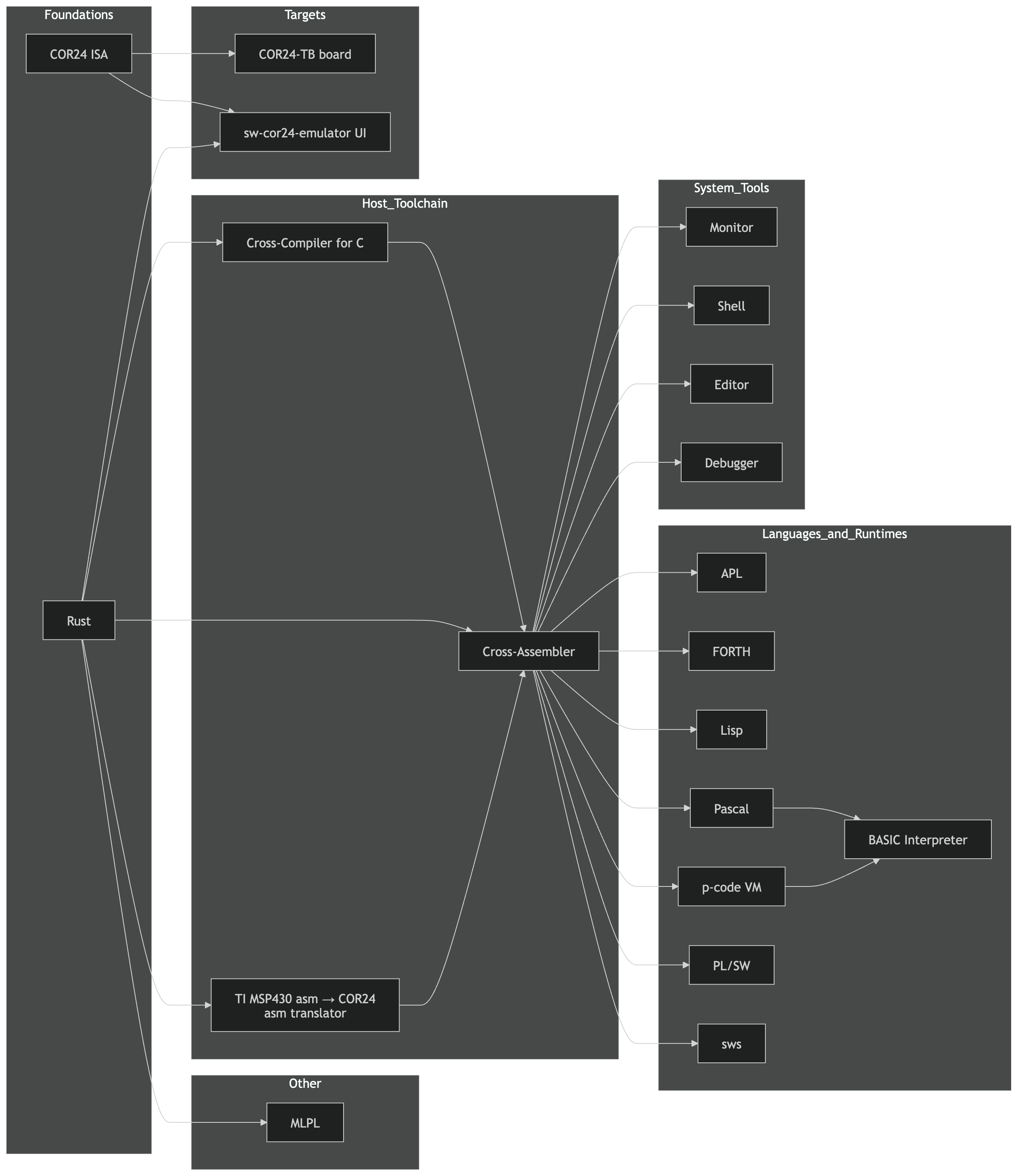
Fixing the C Compiler to Unblock APL
The COR24 APL interpreter is written in C and compiled by
tc24r(a chibicc-inspired C compiler targeting COR24’s 24-bit RISC ISA). APL’s array operations hit several compiler gaps:- Missing features: Certain C constructs that APL’s runtime relied on weren’t yet implemented in tc24r
- Code generation bugs: Edge cases in pointer arithmetic and array indexing produced incorrect COR24 assembly
Each fix in tc24r immediately unblocked APL features that were waiting on correct codegen. The APL REPL now handles more complex array expressions thanks to these fixes.
Extending Pascal to Unblock BASIC
A similar dependency chain on the Pascal side. The COR24 BASIC interpreter runs on a Pascal p-code VM: Pascal source compiles to p-code assembler (
pa24r), links viapl24r, and executes on the COR24 virtual machine. BASIC features that need new p-code instructions require Pascal compiler work first.The Pascal compiler extensions this round added capabilities that BASIC’s string handling and control flow were blocked on. Like the C/APL chain, every Pascal fix cascades into BASIC functionality.
Embedded Tools: Monitor, Shell, and Editor
The COR24 ecosystem also gained progress on three infrastructure tools that make the platform usable as more than a compiler target.
Monitor (
sw-cor24-monitor) is the low-level system monitor—the first thing that runs on COR24 hardware. It provides memory inspection, register dumps, and direct machine-code entry. Think of it as the boot ROM’s interactive console.Script (
sw-cor24-script) is a shell and scripting environment for COR24. It gives the platform a command-line interface for running programs, piping output, and automating tasks—the glue layer between the monitor and the language tools above it.Yocto-Ed (
sw-cor24-yocto-ed) is an Emacs-inspired line editor for COR24. On embedded hardware without a full terminal, a line editor is the practical way to edit source files and configuration. Yocto-Ed borrows Emacs keybindings and concepts (kill ring, incremental search) scaled down to fit in COR24’s memory constraints.All three are works in progress with live demos planned.
Repos and Live Demos
Project GitHub Live Demo agentrail-rs sw-vibe-coding/agentrail-rs N/A APL (integer, embedded) sw-embed/sw-cor24-apl APL REPL BASIC sw-embed/sw-cor24-basic future COR24 Demo Hub sw-embed/web-sw-cor24-demos Demo Hub MLPL (APL2/J/BQN, Rust, float) sw-ml-study/sw-mlpl future Monitor sw-embed/sw-cor24-monitor future Pascal sw-embed/sw-cor24-pascal Pascal Demo PL/SW sw-embed/sw-cor24-plsw PL/SW Demo Script (shell) sw-embed/sw-cor24-script future tc24r (C compiler) sw-embed/sw-cor24-x-tinyc N/A Yocto-Ed (line editor) sw-embed/sw-cor24-yocto-ed future What’s Next
Agentrail-rs: Multi-saga coordination—archived sagas feeding context into new ones, so an agent starting a fresh workstream can learn from completed ones.
MLPL: Parser completion and first interpreter pass. The APL operator semantics validated on COR24 hardware will inform which primitives make it into MLPL’s core.
PL/SW: Macro library for COR24 peripheral access patterns, targeting the MakerLisp hardware and eventually FPGA soft CPUs.
COR24 compilers: Continuing to close gaps in tc24r and the Pascal toolchain as APL and BASIC push further into their respective feature sets.
Sharpen the tools, shorten the chains. Follow for more Sharpen the Saw updates.
Part 5 of the Sharpen the Saw Sundays series. View all parts | Next: Part 6 →
Comments or questions? SW Lab Discord or YouTube @SoftwareWrighter.
- Hardware abstraction:
-
1101 words • 6 min read • Abstract
Bucket List #2: A Landing Page for Software Tools

Resource Link COR24 Software Tools Landing Page Bucket List GitHub Comments Discord The Landing Page
The COR24 Software Tools page is a Yew/WebAssembly single-page application that ties together everything I’ve built for the COR24 24-bit RISC processor. All nineteen tools target the COR24 ISA—assemblers, compilers, interpreters, and system software, all generating or executing COR24 machine code. They’re organized into five groups: foundation tools, cross-compilers, the p-code system, native languages, and system software. Each group has interactive browser demos, documentation, and links to source.
Two weeks ago, most of these existed as scattered repos. Now they have a home, and every one of them is a bucket list item I can point to and say: done, or close to it.
Bucket List Items: Checked Off
Here’s what’s actually built and working, mapped back to the list from Part 1.
Write a Lisp
Tiny Macro Lisp — a Lisp interpreter written in C, targeting COR24. Lexical scoping,
defmacro, closures, and a mark-and-sweep garbage collector. It runs in the browser as a live REPL. This was two bucket list items in one: write a Lisp and implement a garbage collector.I’ve wanted to write a Lisp since I first read Structure and Interpretation of Computer Programs decades ago. The garbage collector was the part I was most nervous about. Turns out, once you have a clear mark phase and a clear sweep phase, it’s not mysterious—it’s just graph traversal with consequences.
Implement a Garbage Collector
See above. Mark-and-sweep, integrated into the Lisp runtime. Every cons cell, every closure, every environment frame is a heap object that gets traced. When the free list runs low, the collector walks the root set and reclaims everything unreachable. Simple, correct, and satisfying to watch in the debugger.
Implement a P-Code VM
P-code VM, Assembler & Linker — the VM is written in COR24 assembly (running on the emulator), with a Rust-based assembler and linker for the toolchain. Plus a Pascal compiler (p24p) that targets the p-code instruction set, and a P-code AOT compiler (pc-aotc) that translates p-code bytecode to native COR24 assembly.
This is straight out of the 1970s UCSD Pascal playbook. A stack-based virtual machine with its own instruction set, a compiler that targets it, and an ahead-of-time compiler that eliminates the interpretation overhead. Three layers of abstraction, all visible and inspectable in the browser.
Design a Systems Programming Language (PL/SW)
PL/SW — inspired by PL/I, targeting COR24. A compiled systems language with structured control flow, typed variables, and direct hardware access. It has its own IDE in the browser.
PL/I was the language IBM designed to replace everything—FORTRAN, COBOL, assembly. It was too ambitious, too complex, and too slow. But the idea of a language that spans systems programming and application programming has always appealed to me. PL/SW is my take on what PL/I might have been if it had been designed for a small machine instead of a mainframe.
Design a Scripting Language (SWS)
SWS — a Tcl-like scripting language for shell and editor automation on COR24. Where PL/SW is for building the system, SWS is for gluing it together. Command substitution, string manipulation, interactive use.
Every system needs a scripting layer. Something you can type at a prompt, something that can automate the editor, something that doesn’t require a compile step. SWS fills that role.
Implement a Monitor
Resident Monitor — boots at address 0, provides program invocation, I/O services, and a command interface. Written in COR24 assembly with some C components. This is the closest thing the COR24 has to an operating system: it loads programs, manages memory regions, and provides system calls.
Implement an Editor
yocto-ed — a minimal modal text editor with a gap buffer implementation. Written in C, compiled with the tc24r cross-compiler. This one is practical: I needed an editor to dogfood the C compiler, so I wrote one. Gap buffers are one of those data structures you hear about but rarely implement yourself.
Write a Compiler (Several, Actually)
- Tiny C Cross-Compiler (tc24r) — compiles a subset of C to COR24 assembly, written in Rust
- Pascal Compiler (p24p) — compiles Pascal to p-code, written in C
- Fortran Compiler — translates Fortran to COR24 assembly, written in C
- P-code AOT Compiler (pc-aotc) — translates p-code bytecode to native COR24 assembly
- Native Assembler (as24) — runs on the COR24 itself, part of the self-hosting toolchain
Five compilers/translators. Each one taught me something different about parsing, code generation, register allocation, and the gap between source language semantics and machine capabilities.
Implement an Interpreter
Beyond the Lisp interpreter, there’s also:
- Forth IDE — a direct-threaded code Forth with dictionary browsing and stack inspection
- APL Interpreter (apl-sw) — integer-only APL with rank-2 arrays
- BASIC Interpreter — classic BASIC with line numbers, GOTO/GOSUB, string variables
Four interpreters across four very different language paradigms: functional (Lisp), concatenative (Forth), array-oriented (APL), and imperative (BASIC).
Still on the List
A few items from Part 1 aren’t checked off yet:
- Debugger — a source-level debugger is planned but not yet implemented
- Shell — the monitor handles basic command dispatch, but a proper shell with pipes and redirection is future work
- Linker — the p-code linker exists, but a general-purpose native linker is still to come
The Vibe-Coding Part
All of this was built with AI assistance via agentrail-rs. The pattern: I describe what I want at an architectural level—“implement a mark-and-sweep garbage collector for the Lisp runtime”—and the AI writes the implementation. I review, test, redirect, and iterate. The landing page itself is a Yew SPA compiled to WebAssembly with Trunk, using the Catppuccin Mocha theme.
Two weeks. Nineteen tools. One person, operating as architect and project manager rather than line-by-line coder.
This is what retirement plus AI looks like. The bucket list is getting shorter.
Previous: Bucket List #1: Things I’ve Always Wanted to Build — the full list.
Part 2 of the Bucket List series. View all parts | Next: Part 3 →
Comments or questions? SW Lab Discord or YouTube @SoftwareWrighter.
-
1237 words • 7 min read • Abstract
Saw #4: All Together Now --- Emacs Meets the Multi-Agent Orchestra

Why Sharpen the Saw? — The name comes from Covey’s Habit 7: stop cutting long enough to sharpen the blade. This series is the weekly checkpoint where I step back from feature work and invest in the tools themselves—smoother editor integration, better agent coordination, less friction between the moving parts. Four weeks in, the compound interest is showing.
Resource Link pjmai-rs sw-cli-tools/pjmai-rs reg-rs sw-cli-tools/reg-rs All Together Now sw-vibe-coding/all-together-now Prior Post Saw #3: agentrail-rs — From Walking Skeleton to Dual Memory Comments Discord Emacs Meets the CLI: pjmai-rs
pjmai-rs is a project manager that maintains a stack-based navigation history, groups, and per-project metadata. It works well from the terminal, but Emacs
shell-modehas a blind spot: when the CLI changes directories via exit-code signaling, Emacs doesn’t updatedefault-directory. File completion breaks. Dired opens the wrong place.The new
pjmai.elpackage (376 lines) solves this by calling the binary directly from Elisp and managing per-project shell buffers wheredefault-directoryis correct from the start.What It Does
Everything lives under the
C-c pprefix:Key Action C-c p cChange project (opens/switches shell) C-c p lList projects C-c p sShow current project C-c p pPush to stack and switch C-c p oPop from stack C-c p dOpen project in dired C-c p aAdd project C-c p eEdit project metadata C-c p gGroup commands (list, show, prompt) Each project gets a dedicated shell buffer (
*pjmai:projectname*) with the correct working directory set before the shell spawns. Tab completion just works. The shell function is pluggable—#'shellby default, but#'vtermor#'eshellare configurable.25 ERT tests cover the CLI interface, JSON parsing, project completion, shell buffer management, and keymap structure.
Emacs Meets the CLI: reg-rs
reg-rs is a regression testing tool that captures command output and diffs against baselines. Like pjmai-rs, it had great terminal ergonomics but required context-switching away from Emacs.
my-reg-rs.el(208 lines) puts regression testing underC-c r:Key Action C-c r rRun all tests C-c r vRun verbose C-c r lList tests C-c r sShow test details C-c r uUpdate/accept baselines C-c r aAdd new test C-c r RRerun last command Output goes to
compilation-modebuffers, sonext-errornavigation works naturally. The package auto-detects the project root by checking forwork/reg-rs/,.rgt/.tdbfiles, or falling back toproject.el.All Together Now: A Multi-Agent Program Manager
The bigger project this week. I’ve been running multiple Claude Code instances across repos and the coordination overhead was becoming the bottleneck—switching tabs, manually checking wikis, copying context between agents. All Together Now (ATN) is a Program Manager that owns the agent terminals and provides a unified control plane.
The Architecture
ATN runs as an Axum HTTP server that spawns N agents via
portable-pty, streams their terminal output through SSE to a browser dashboard, and maintains a shared wiki for coordination state.
Four Phases in One Session
Phase What Tests 0+1 PTY session management—spawn, read/write, Ctrl-C, transcripts 5 integration tests 2 Minimal web UI—SSE streaming, xterm.js terminal widget Working end-to-end 3 Multi-agent dashboard—N agents, per-agent state machine, responsive grid 3-agent demo (alice, bob, carol) 4 Wiki integration—REST CRUD, ETag-based CAS, seeded coordination pages 8 unit tests 29 tests pass across the workspace. Zero clippy warnings.
The Six Crates
Crate Lines Role atn-core~300 Domain types: AgentConfig, AgentState, events, routing atn-pty~500 PTY sessions, serialized writer queues, state tracker atn-server~270 Axum HTTP/SSE server, static UI atn-ui~200 Yew WASM components (dashboard, wiki browser) atn-wiki~300 File-backed wiki with CAS from wiki-rs atn-trail~200 Agentrail integration for workflow tracking Why PTY Ownership Matters
The key insight: if the Program Manager owns the pseudo-terminals, it can:
- Stream output to a web dashboard without agents knowing
- Inject commands into agent sessions (serialized, no interleaving)
- Detect state by parsing output (prompt markers, idle timeouts, question detection)
- Log transcripts for debugging and replay
The serialized writer queue per agent prevents input corruption when multiple sources (human, coordinator, macros) write to the same terminal.
Wiki as Coordination Layer
ATN seeds five coordination pages on startup:
Page Purpose Coordination/GoalsTeam objectives Coordination/AgentsWho is doing what (auto-updated) Coordination/RequestsInter-agent feature/bug requests Coordination/BlockersDependency tracking Coordination/LogAppend-only event timeline The wiki uses ETag-based Compare-and-Swap from the wiki-rs project, so concurrent agent writes get conflict detection instead of silent data loss.
What’s Next
ATN Phase 5: Message routing—agents write JSON to an outbox, the PGM routes push events to the correct target agent or escalates to human review.
Emacs packages: Phase 2 additions—
transientmenus for discoverability, completion annotations showing project paths and languages.Emacs as ATN frontend: The pjmai-rs and reg-rs Emacs packages prove the pattern—call a Rust binary from Elisp, parse structured output, manage buffers. The same approach will give Emacs users a native ATN interface: agent status, wiki edits, and command injection without leaving the editor.
Tying it together: ATN + agentrail-rs integration, where each agent’s workflow progress is visible in the dashboard (and eventually in Emacs) and skills/experiences flow between sessions.
Better tools, better integration. Follow for more Sharpen the Saw updates.
Part 4 of the Sharpen the Saw Sundays series. View all parts | Next: Part 5 →
Comments or questions? SW Lab Discord or YouTube @SoftwareWrighter.
-
1479 words • 8 min read • Abstract
TBT #8: wiki-rs --- Six Wikis, One Engine, Thirty Years of History

Resource Link Live Demo wiki-rs (3 client-side wikis) Source GitHub Video wiki-rs: Six Wikis, One Engine 
Agent Wiki Sample synced page Comments Discord The Throwback
I was a reader of Ward Cunningham’s original WikiWikiWeb in the late 1990s. The concept was radical at the time: a website where any visitor could edit any page, with no approval process, no gatekeeping. Pages linked to each other with
CamelCasewords. If a page didn’t exist, the link showed up differently—click it, and you created it. The entire system ran on flat files.In the early 2000s at Sun Microsystems, I started installing wikis for my teams. The first was TiKi, a Ruby-based wiki—CGI scripts, flat-file storage, pre-Rails era. It was fragile but functional. Later I moved to VQWiki, a Java servlet-based wiki that could deploy as a WAR file and supported both file and database storage. VQWiki was reliable enough for engineering teams to depend on.
Along the way I used TiddlyWiki for personal projects—an entire wiki in a single HTML file, no server required. And these days I use GitHub Wikis for public projects, which are just git-backed markdown repositories.
Each of these represents a different answer to the same question: where do the pages live?
The Storage Question
Every wiki engine has to answer this:
Era Engine Storage Trade-off 1995 WikiWikiWeb Flat files Simple, no dependencies, no versioning ~2002 TiKi (Ruby) CGI + flat files Easy deployment, fragile under load ~2002 VQWiki (Java) Servlet + file/DB hybrid Reliable, but heavyweight 2004 TiddlyWiki Single HTML file Zero server, but limited scalability Modern GitHub Wiki Git repository Full versioning, but requires git The storage architecture determines everything about a wiki: how it scales, how it versions, how it deploys, whether it needs a server, and how portable the data is.
wiki-rs: Six Approaches in Rust
I wanted to build all of these approaches in one codebase to see how they compare. wiki-rs implements six wiki variants, all sharing the same UI and wiki engine, differing only in storage:
Variant Storage Server Required? Demo Ephemeral In-memory HashMap No Live Browser Memory localStorage No Live Export/Import JSON file download/upload No Live Server File Axum + flat .mdfilesYes Local Server DB Axum + SQLite Yes Local Server Git Axum + git commits Yes Local The three client-side wikis run entirely in the browser via WebAssembly—no server, no installation. The three server wikis use Axum and require a local backend.
Shared Engine, Pluggable Storage
The architecture uses two storage traits:
WikiStorage(sync) — for WASM frontends where async isn’t availableAsyncWikiStorage(async) — for server backends
Each wiki variant is a thin wrapper (~30 lines) that implements the appropriate trait and calls the shared
render_wiki()entry point. The wiki engine—parsing, rendering, link resolution, editing—is identical across all six.The full codebase is 11 crates in a Cargo workspace, totaling ~2,600 lines of Rust.
Wiki Engine Features
The engine handles the essentials:
- Wiki links:
[[PageName]]and[[PageName|display text]] - Red links: nonexistent pages show as red; clicking creates the page
- Markdown: headings, bold, italic, code blocks, lists (via pulldown-cmark)
- Page aging: five visual tiers (Fresh, Recent, Stale, Old, Ancient) based on when a page was last edited—complete with yellowing, parchment gradients, and folded-corner effects
- Sub-wiki theming: five color themes detected by page title prefix (e.g.,
Tech/Rustgets the Ocean theme) - XSS protection: raw HTML filtered out; wiki links inside backticks aren’t expanded
Import: VQWiki and TiddlyWiki
Since I have old wiki content in both VQWiki and TiddlyWiki formats, the project includes markup converters for both:
- VQWiki importer: converts VQWiki’s custom markup (
!!!headings,'''bold''',[link|url]) to standard wiki markdown - TiddlyWiki importer: extracts tiddlers from TiddlyWiki HTML files and converts their markup
Both converters have test suites validating the markup transformations.
What I Learned
Building six variants of the same wiki clarified the trade-offs:
Ephemeral is great for demos and testing. No persistence means no state bugs, but close the tab and everything’s gone.
Browser localStorage is surprisingly useful for personal wikis. No server, data persists across sessions, and the 5-10 MB limit is plenty for text. The limitation is portability—the data lives in one browser on one machine.
Export/Import solves portability. Download the wiki as JSON, email it, upload it elsewhere. But there’s no real-time versioning.
Server File is the closest to the original WikiWikiWeb. Flat
.mdfiles that you can read, grep, and back up with any tool. Simple and transparent, but no built-in versioning.Server SQLite adds transactions, queries, and atomic operations. The trade-off is opacity—your wiki is inside a database file, not human-readable files.
Server Git is the most powerful. Every edit is a git commit with full history, diff, blame, and branch support. But it’s also the most complex and has the highest overhead per edit.
From Throwback to AI Coordination
A pattern I follow with these projects: think of a cool technology I used in the past, figure out how to recreate it in some demonstrable way, and think about how it could benefit from AI features—or how an AI agent could benefit from a modern tool based on the technology.
While working on an ambitious multi-repo project with multiple AI agents, I needed to act as coordinator between agents to implement a major refactoring. Each agent worked in its own repo, but they had shared dependencies, sequencing constraints, and status updates that needed to flow between them. I was the bottleneck—manually relaying context from one agent session to another.
I wondered if there was a way to delegate this coordination to an AI agent. And then I realized: my server-based wikis were already designed to share structured information. A wiki could serve as the shared state layer—goals, dependencies, requests, status, context—all on editable pages that any agent could read and update.
The problem: multiple agents editing the same wiki pages simultaneously will corrupt each other’s work. So I added a Compare-and-Swap (CAS) API to the wiki server. Each edit includes the page’s current version hash. If the page changed since the agent last read it, the write is rejected and the agent must re-read, merge, and retry. This gives you serialized concurrent edits without locking—the same pattern databases use for optimistic concurrency.
Then I needed a way to monitor and document what the agents were doing. So I added a tool to export the CAS wiki as a snapshot to a GitHub Wiki. Now the coordination state is visible, versioned, and browsable on GitHub—a living record of how the agents collaborated.
During early testing, one agent overwrote another agent’s request on a shared page—a classic lost-update problem. The affected agent eventually noticed (its request had vanished), but the damage was done. That’s exactly what CAS prevents at the API level. But it also showed that structural serialization isn’t enough—agents can still make semantic conflicts even when their writes don’t collide. So I asked the wiki-rs agent to add a feature to help serialize semantic changes too, ensuring agents merge intent rather than just bytes.
This is where throwback meets frontier: a thirty-year-old concept (the wiki), rebuilt in Rust, extended with concurrency primitives, and put to work as infrastructure for multi-agent AI coordination.
Quality
The project was built with a TDD red/green/refactor process:
- 50 integration tests across unit, API, and Playwright browser tests
- Zero clippy warnings
- 69/69 on the sw-checklist quality gates
The wiki is thirty years old and still the simplest way to organize knowledge. What’s on yours?
Part 8 of the Throwback Thursday series. View all parts | Next: Part 9 →
Comments or questions? SW Lab Discord or YouTube @SoftwareWrighter.
-
1201 words • 7 min read • Abstract
ML Frontier #04: Is Chain of Thought Real?

Fourth ML Frontier episode. In 2022, Chain of Thought changed how we think about AI reasoning. By 2026, the question has shifted from “how to make CoT better” to “is it real reasoning at all?”
Resource Link Papers 10 papers (2024–2026) Video ML Frontier 4: Is CoT Real? 
Comments Discord What Chain of Thought Promised
Wei et al. (2022) showed that prompting language models to “think step by step” dramatically improved performance on math, logic, and multi-step reasoning tasks. The idea was simple: instead of jumping straight to an answer, generate intermediate reasoning steps. The model explains its work, and the answer improves.
This became the foundation for everything from coding assistants to scientific reasoning pipelines. But a deeper question was always lurking: are those reasoning steps real?
The Faithfulness Problem
Recent research shows models can produce plausible-looking reasoning steps that don’t reflect their actual internal computation. The chain of thought looks like reasoning—it has logical connectives, intermediate conclusions, references to the problem—but the model may have arrived at the answer through entirely different internal pathways.
This is the faithfulness gap. A model’s visible reasoning trace can be:
- Post-hoc rationalization — constructing a justification after already deciding the answer
- Biased by surface features — following patterns in the prompt rather than the problem structure
- Unfaithful to internal state — the actual computation happening in the model’s hidden layers doesn’t match the text it generates
“Reasoning Models Don’t Always Say What They Think” (arXiv 2505.05410) shows that even models specifically trained to reason via CoT produce traces that are often unfaithful to their actual decision process. A March 2026 follow-up, “Reasoning Models Struggle to Control their Chains of Thought” (arXiv 2603.05706), goes further: models can’t reliably steer or suppress their reasoning traces even when instructed to. And “Diagnosing Pathological Chain-of-Thought in Reasoning Models” (arXiv 2602.13904) catalogs specific failure modes where CoT reasoning becomes actively pathological.
The implication is uncomfortable: when a model shows you its “thinking,” you can’t assume it’s showing you how it actually thinks.
CoT Is Task-Dependent
The research also reveals that Chain of Thought isn’t universally beneficial. It helps with:
- Math and arithmetic — multi-step calculations benefit from intermediate results
- Multi-hop logic — problems requiring sequential deductions
- Complex planning — tasks with dependencies between steps
But CoT can actually hurt performance on:
- Pattern recognition — tasks where the answer is immediate/intuitive
- Simple classification — forcing step-by-step reasoning adds noise
- Tasks with misleading structure — when the “obvious” reasoning path leads away from the correct answer
A 2024 meta-analysis, “To CoT or not to CoT?” (arXiv 2409.12183), confirms this systematically: CoT provides negligible or negative benefit on many task types including commonsense reasoning and factual retrieval. The blanket advice of “always use Chain of Thought” is wrong. The right approach depends on the task.
Adaptive Reasoning: Knowing When to Think
The field is moving toward conditional reasoning—models that decide when to think step by step and when to skip it. Wang and Zhou (2024) showed that chain-of-thought reasoning can emerge from models without explicit prompting, suggesting the capability is latent rather than purely prompt-dependent.
This points toward a future where models dynamically allocate reasoning effort:
- Simple questions get immediate answers
- Complex questions trigger step-by-step decomposition
- Ambiguous questions get clarifying sub-questions
“s1: Simple Test-Time Scaling” (arXiv 2501.19393) demonstrates this with budget-forcing—a simple mechanism to control how much reasoning a model performs at test time, truncating or extending thinking adaptively. “Outcome-Based RL Provably Leads Transformers to Reason” (arXiv 2601.15158) shows that RL training can teach transformers when reasoning is needed, not just how to reason. The model itself becomes the judge of how much thinking a problem requires.
Latent Reasoning: Thinking Without Showing
Some of the most interesting current work explores latent reasoning—models that reason internally without generating visible steps. Instead of producing a text trace, the model uses its internal representations to perform multi-step computation within the forward pass.
This connects to research on:
- Implicit chain of thought — reasoning encoded in hidden states rather than output tokens
- Pause tokens — giving models extra computation steps without requiring text output
- Internal scratchpads — dedicated hidden-state computation that doesn’t appear in the response
COCONUT (arXiv 2412.06769) demonstrates this concretely: LLMs reason using continuous hidden states as “thoughts” instead of generating discrete tokens. Two 2026 papers push further: “Latent Chain-of-Thought as Planning” (arXiv 2601.21358) decouples reasoning from verbalization entirely, and “Latent Reasoning with Supervised Thinking States” (arXiv 2602.08332) trains models to reason through supervised internal states.
If latent reasoning works at scale, it could offer the accuracy benefits of CoT without the token cost or the faithfulness problem—because there’s no visible trace to be unfaithful.
CoT as Part of an Ecosystem
Chain of Thought is no longer a standalone technique. It’s one component in a broader ecosystem:
Component Role CoT Step-by-step decomposition Tool use Offload computation to external systems Reflection Self-critique and error correction Planning loops Multi-turn strategy with backtracking Reinforcement learning Reward signals for reasoning quality This makes CoT the bridge concept between language models as predictors (next token), as reasoners (multi-step logic), and as agents (goal-directed behavior). Understanding where CoT works and where it breaks is essential for building systems that combine all three.
The Open Questions
Question Status Is CoT faithful to internal computation? Evidence says often not When should models use CoT? Task-dependent; adaptive approaches emerging Can models reason without visible steps? Latent reasoning research is promising Does CoT scale with model size? Yes, but with diminishing returns on simple tasks Will CoT survive as a technique? Likely evolves into adaptive/latent forms Papers
Date Paper Link Jan 2022 Chain-of-Thought Prompting Elicits Reasoning in Large Language Models arXiv 2201.11903 Sep 2024 To CoT or not to CoT? CoT Helps Mainly on Math and Symbolic Reasoning arXiv 2409.12183 Dec 2024 Training LLMs to Reason in a Continuous Latent Space (COCONUT) arXiv 2412.06769 Jan 2025 s1: Simple Test-Time Scaling arXiv 2501.19393 May 2025 Reasoning Models Don’t Always Say What They Think arXiv 2505.05410 Jan 2026 Outcome-Based RL Provably Leads Transformers to Reason arXiv 2601.15158 Jan 2026 Latent Chain-of-Thought as Planning arXiv 2601.21358 Feb 2026 Latent Reasoning with Supervised Thinking States arXiv 2602.08332 Feb 2026 Diagnosing Pathological Chain-of-Thought in Reasoning Models arXiv 2602.13904 Mar 2026 Reasoning Models Struggle to Control their Chains of Thought arXiv 2603.05706
Is the reasoning real, or just a good story? Follow for more ML Frontier episodes exploring research at the edge.
Part 4 of the Machine Learning Frontier series. View all parts | Next: Part 5 →
Comments or questions? SW Lab Discord or YouTube @SoftwareWrighter.
-
1357 words • 7 min read • Abstract
Saw #3: agentrail-rs --- From Walking Skeleton to Dual Memory

Resource Link Repo sw-vibe-coding/agentrail-rs Prior Post Saw #2: reg-rs, avoid-compaction, and agentrail Related ML Frontier #02: ICRL Related AI Tools #1: XSkill Comments Discord The Problem agentrail Solves
AI coding agents lose operational knowledge between sessions. An agent might figure out the right sequence of commands for a complex task—TTS generation, video compositing, file manipulation—then lose that knowledge when the session ends. Next time, it starts from scratch. Sometimes it succeeds. Sometimes it improvises and fails.
agentrail-rs gives agents structured handoffs, deterministic step execution, and in-context reinforcement learning so they succeed on first attempts instead of guessing.
What’s Working: Beyond the Walking Skeleton
Phase 0 through Phase 5 (partial) are implemented. The CLI has 8 commands that manage the full saga lifecycle:
agentrail init my-project      # Create a new saga
agentrail plan                  # Show the step sequence
agentrail next                  # Get instructions for the next step
agentrail begin step-name       # Mark a step as in-progress
agentrail complete step-name    # Mark a step as done
agentrail status                # Show saga state
agentrail history               # Show completed steps
agentrail abort                 # Cancel the saga
Everything persists to a
.agentrail/directory: TOML configs, JSON trajectories, JSONL session snapshots. The 24 integration tests all pass, and pre-commit quality gates enforce formatting, lints, and test coverage.Two-Layer Architecture
The architecture separates the generic engine from domain-specific knowledge:
Layer 1 (this repo) — task-agnostic inference-time learning:
- Workflow state machine (sagas with typed steps)
- Dual memory following the XSkill pattern: skills (strategic workflow documents) and experiences (tactical per-run records)
- ICRL injection: retrieve successful experiences and inject them into agent prompts
- Distillation: analyze experience batches, generate and update skill documents
Layer 2 (separate repos, future) — domain-specific knowledge:
- Per-domain repos (e.g.,
agentrail-domain-media,agentrail-domain-rust) - Skill documents, curated experience libraries, executor implementations, validators
- Optional knowledge graphs for reward signals
The separation means the engine never changes when you add a new domain. You just create a new Layer 2 repo with the right skill files and executors.
The XSkill Connection
The dual-memory pattern comes directly from the XSkill paper (arXiv 2603.12056). Their ablation analysis shows that removing either skills or experiences hurts performance—you need both.
In agentrail-rs:
Memory Type What It Stores How It’s Used Skills Structured workflow documents for a class of tasks Injected into agentrail nextto give the agent a strategic playbookExperiences Tactical records from past runs (what worked, what failed) Injected into agentrail nextto show the agent what succeeded beforeWhen you run
agentrail next, it retrieves relevant skills and past trajectories and includes them in the output. The agent sees both how to approach this kind of task (skill) and what actually worked last time (experience).Research Foundations
The architecture maps to specific research:
Research How It’s Applied ICRL (Decision Transformer, Reflexion, Voyager) Agents learn from trajectory examples in context, not weight updates XSkill (dual memory) Skills + experiences, both necessary Knowledge Graphs as Reward Models Graph edges as verifiable reward signals (Phase 4) Sleepy Coder experiment LoRA fine-tuning couldn’t beat baseline, validating inference-time approach The Sleepy Coder result was pivotal. I’d spent weeks trying to fine-tune a small model for my specific agent tasks. The fine-tuned model performed worse than the base model with good prompts. That’s what pushed me toward ICRL: don’t change the model’s weights, change what it sees in context.
Implementation Progress
Phase Description Status 0 Walking skeleton (CLI, persistence, tests) Done 1 ICRL core loop (task types, trajectory retrieval, experience recording) Done 2 Dual memory (Skill/Experience types, injection, distillcommand)Done (2a, 2d) 3 Domain repo support (registry, executors, validators) Done (partial) 4 Knowledge graph validation (graph-based rewards) Planned 5 Hybrid orchestrator (auto-advance deterministic steps, escalate semantic work) Done (partial) Phase 1 added
task_typeto step configs, trajectory retrieval inagentrail next, and experience recording with--reward/--actionsflags oncomplete. Phase 2a introduced theSkilltype with TOML storage and injection intonextoutput. Phase 2d added thedistillcommand that analyzes experience batches to generate skill documents. Phase 3 brought the domain registry, executor trait, and validator trait. Phase 5 implemented the hybrid orchestrator loop where deterministic steps auto-advance and semantic work gets escalated to the agent.What remains: Phase 2b/2c (enriched Experience type, experience retrieval by embedding), Phase 3 completion (first real domain repo), and Phase 4 (knowledge graph rewards).
Vibe Coding Projects
agentrail-rs is being developed by building extensions to these vibe coding projects—each one is a real test case for domain-specific skills and experiences.
Project Link cor24-rs sw-embed/cor24-rs — COR24 assembly emulator (Rust, WASM, embedded) tc24r sw-vibe-coding/tc24r — C compiler for COR24 (C, compiler design, browser) wiki-rs sw-vibe-coding/wiki-rs — Wiki implementations (Rust, web UI) What’s Next: Domain-Specific Layer 2
The engine (Layer 1) is functional. The next challenge is building real Layer 2 domain repos and proving the architecture works on actual projects. This week I’m testing it against three new projects:
- A C compiler running in a browser — requires WebAssembly compilation skills
- A Macro Lisp implemented in C — requires C development and language implementation skills
- The Macro Lisp running inside a browser — combines all of the above with Web UI skills
This is a deliberate stress test. Each project demands different domain expertise: C, Rust, Lisp, and Web UI. If agentrail-rs can carry skills and experiences across these domains and help the agent succeed on first attempts, the architecture works. If not, I’ll learn where it breaks.
Crate Layout
The project is a Cargo workspace (edition 2024) with clean separation:
Crate Role agentrail-coreDomain types: SagaConfig, StepConfig, Skill, Trajectory, HandoffPacket, JobSpec agentrail-storeFile-based persistence ( .agentrail/), skill and trajectory storageagentrail-cliBinary with 8 commands + distillagentrail-execDeterministic step executors with domain registry agentrail-validateOutput validators with domain registry Papers
Date Paper Link Feb 2025 OmniRL: In-Context RL Across Multiple Tasks arXiv 2502.02869 Jan 2026 Knowledge Graphs are Implicit Reward Models arXiv 2601.15160 Mar 2026 XSkill: Continual Learning from Experience and Skills arXiv 2603.12056 Mar 2026 An Alternative Trajectory for Generative AI arXiv 2603.14147
Better tools, better agents. Follow for more Sharpen the Saw updates.
Part 3 of the Sharpen the Saw Sundays series. View all parts | Next: Part 4 →
Comments or questions? SW Lab Discord or YouTube @SoftwareWrighter.
-
1943 words • 10 min read • Abstract
Embedded #2: COR24-RS --- Learn Assembly in Your Browser

Resource Link Live Demo COR24 Assembly Emulator Source GitHub Video Browser-Based Assembly: COR24 RISC Emulator in Rust 
MakerLisp makerlisp.com (COR24 creators) COR24 Soft CPU FPGA Implementation COR24 Dev Board Hardware Kit Comments Discord
What is COR24?
COR24 (C-Oriented RISC 24-bit) is a soft CPU architecture designed by MakerLisp. The design priorities were simplicity, speed, and a good impedance match to C compilers on low-density FPGAs—no legacy requirements, no committee compromises. The “C-Oriented” in the name is literal: architectural decisions were informed by what a practical C compiler needs from this class of processor.
Origin Story
MakerLisp developed COR24 as a replacement for the eZ80, which was the best option they could find for their class of small embedded problems. During the pandemic-era chip shortage, mass-market microcontrollers became unavailable, so they designed their own CPU for FPGAs. The result: a 24-bit RISC architecture that runs at 101 MHz on inexpensive Lattice FPGAs—a simple, fast, and rational alternative built from the ground up with no legacy baggage.
The CPU is written in Verilog and released under the MIT license. It’s both a practical embedded solution for small computing problems and an excellent architecture for learning CPU fundamentals. You can build your own hardware implementation or use the browser emulator to explore the architecture.
Architecture Overview
COR24 keeps things simple. Three general-purpose registers, five special-purpose registers, one condition flag, and instructions that are 1, 2, or 4 bytes long.
Registers
Register Purpose r0 General purpose / return value r1 General purpose / return address r2 General purpose fp Frame pointer (special) sp Stack pointer (special) z Constant zero (compare instructions only) iv Interrupt vector (special) ir Interrupt return (special) Only r0, r1, and r2 are truly general-purpose. The named registers (fp, sp, z, iv, ir) have dedicated roles. The z register provides a constant zero accessible only in compare instructions (
ceq r0, z,clu z, r0,cls r0, z)—it is not a general-purpose register and cannot be used in mov, ALU, or load/store instructions. The architecture uses a separate condition flag (C) set by compare instructions and tested by branch instructions.Memory Model
- 24-bit address space (16 MB addressable)
- Byte-addressable with little-endian ordering
- Memory-mapped I/O at 0xFF0000 - 0xFFFFFF
- Stack grows downward (standard convention)
Instruction Categories
Category Instructions Arithmetic add,sub,mulLogic and,or,xorShifts shl,sra,srlCompare ceq,cls,cluBranch bra,brf,brtJump jmp,jalLoad la,lc,lcu,lb,lbu,lwStore sb,swStack push,popMove mov,sxt,zxtInstructions are 1, 2, or 4 bytes (never 3). Register-only operations are compact (1 byte). Loading 8-bit constants (sign- or zero-extended) uses 2-byte instructions (
lc,lcu). Loading full 24-bit values—whether addresses or integers that don’t fit in 8 bits—requires 4-byte instructions (la). Note: data words are 3 bytes (24-bit), but instruction encoding never uses 3 bytes.The Dev Board
The COR24-TB dev board exposes the CPU’s I/O in a hands-on layout. The S2 button is a user switch—press it and the CPU sees an input event your assembly code can poll or respond to. D2 is a user LED wired to a memory-mapped output address, so your code can toggle it directly with a store instruction. The board breaks out UART connectors for serial communication, with hardware support for an internal interrupt when data arrives—meaning your program doesn’t have to busy-wait on the serial port. Beyond these, the board has six additional GPIO pins intended for a four-wire SPI interface and a two-wire I2C bus. MakerLisp is actively developing bit-bang I2C support (temperature sensor reading is next), followed by an I2C real-time calendar clock, a 4-position 7-segment display via SPI, and SD card access via SPI. A Reset button and Power LED round out the essentials.
The emulator models the S2 button, D2 LED, and UART with interrupt support, so programs written for the browser run the same way on real hardware.
The Browser Emulator
cor24-rs brings COR24 to the web using Rust compiled to WebAssembly. No downloads, no setup—just open the page and start coding.
Features
- Three Tabs - Assembly, C, and Rust pipelines, all running on the same COR24 CPU
- Interactive Assembly Editor - Syntax highlighting, error messages, line numbers
- Step-by-Step Execution - Execute one instruction at a time with log-scale speed control
- Register & Memory Viewer - Watch CPU state change in real-time with highlighted changes
- Instruction Trace - Last 100 executed instructions visible in the web UI
- 11 Assembler Examples - Pre-loaded programs including Blink LED, Fibonacci, Countdown, Variables, and Assert
- 12 Rust Pipeline Demos - From simple add to UART echo with interrupts
- 2 C Pipeline Examples - Fibonacci and Sieve of Eratosthenes via MakerLisp’s CC24 compiler
- Coding Challenges - Test your assembly skills with suggested exercises
- ISA Reference - Complete instruction documentation inline with CPU state, interrupts, and memory map
- Interactive Tutorial - Comprehensive introduction covering registers, instructions, I/O, and idioms
- Self-Test Mode -
?selftestURL parameter runs all 15 examples automatically with pass/fail reporting - Animated Tours -
?showme-asm,?showme-c,?showme-rustwalk through each pipeline - Realistic UART Timing - TX busy for 10 cycles per character; dropped characters when writing without polling
Example: Fibonacci
Here’s a recursive Fibonacci implementation in COR24 assembly:
_fib:
        push    fp              ; Save frame pointer
        push    r2              ; Save r2
        push    r1              ; Save return address
        mov     fp,sp           ; Set up frame
        add     sp,-3           ; Local variable space
        lw      r2,9(fp)        ; Load argument n

        lc      r0,2            ; Load constant 2
        cls     r2,r0           ; Compare n < 2
        brf     L17             ; Branch if false

        lc      r0,1            ; Return 1
        bra     L16             ; Jump to epilogue

L17:
        mov     r0,r2           ; r0 = n
        add     r0,-1           ; r0 = n - 1
        push    r0              ; Push argument
        la      r0,_fib         ; Load fib address
        jal     r1,(r0)         ; Call fib(n-1)
        add     sp,3            ; Clean up argument
        sw      r0,-3(fp)       ; Save result

        mov     r0,r2           ; r0 = n
        add     r0,-2           ; r0 = n - 2
        push    r0              ; Push argument
        la      r0,_fib         ; Load fib address
        jal     r1,(r0)         ; Call fib(n-2)
        add     sp,3            ; Clean up argument
        lw      r1,-3(fp)       ; Load fib(n-1)
        add     r0,r1           ; r0 = fib(n-1) + fib(n-2)

L16:
        mov     sp,fp           ; Restore stack
        pop     r1              ; Restore return address
        pop     r2              ; Restore r2
        pop     fp              ; Restore frame pointer
        jmp     (r1)            ; Return
This demonstrates the full calling convention: prologue/epilogue, argument passing via stack, and recursive calls.
Command Line Tools
Beyond the browser emulator, cor24-rs includes CLI tools for local development:
# Assemble and run in the debugger
cor24-dbg program.s

# Or assemble and run directly
cor24-run program.s

# With LED visualization
cor24-run program.s --leds
The CLI debugger (
cor24-dbg) supports breakpoints, step execution, UART I/O, LED/button simulation, and instruction trace. The--uart-never-readyflag forces TX to never clear, useful for testing polling behavior.
Rust to COR24 Pipeline (Experimental)
The project includes experimental support for compiling Rust to COR24:
Rust (.rs) → WASM (.wasm) → COR24 Assembly (.s) → Binary
            ↑               ↑
         rustc          wasm2cor24
        (standard)       (this project)
Write embedded Rust with
#![no_std], compile to WebAssembly, then translate to COR24 assembly. The wasm2cor24 translator handles the stack-based IR conversion.This approach leverages Rust’s existing toolchain—no compiler modifications needed. The wasmparser crate handles WASM parsing, and COR24’s stack-oriented design maps reasonably well from WASM’s stack machine.
Why Learn Assembly?
Even if you never write production assembly, understanding it changes how you think about code:
- Performance intuition - Know what your high-level code compiles to
- Debugging - Read crash dumps and disassembly when things go wrong
- Security - Understand buffer overflows, ROP chains, exploitation
- Embedded systems - Some hardware requires low-level access
- Appreciation - Respect the layers beneath your abstractions
COR24 is simple enough to fit in your head but realistic enough to represent real CPU design patterns. And unlike purely educational architectures, it’s also a practical platform for small embedded problems—the kind of work that used to require an eZ80 or similar microcontroller.
Implementation Details
The emulator core is written in Rust, compiled to WebAssembly via Trunk. Key components:
Module Purpose cpu/state.rsCPU state management (registers, memory, flags) cpu/executor.rsInstruction execution engine with realistic UART timing cpu/decode_rom.rsInstruction decode ROM (extracted from hardware Verilog) assembler.rsTwo-pass assembler with as24-compatible syntax enforcement challenge.rsCoding challenge definitions selftest.rsAutomated test runner for all 15 examples app.rsYew-based web application (3 tabs, animated tours) The decode ROM is particularly interesting—it’s extracted directly from the hardware Verilog implementation, ensuring the emulator matches the real CPU behavior exactly.
Try It Yourself
Live Demo: sw-embed.github.io/cor24-rs
The demo includes:
- Pre-loaded example programs
- Interactive tutorials
- Coding challenges with automated verification
- Complete ISA reference
Start with the “Hello World” example, then work through the challenges. By the time you complete them, you’ll understand registers, memory, stack operations, and function calls.
Key Takeaways
- COR24 is a real CPU - Designed for FPGAs, runs at 101 MHz, MIT licensed, practical for embedded work
- cor24-rs makes it accessible - Browser-based, no installation required
- Assembly isn’t scary - With good tools, you can see every step
- Rust + WASM works - The entire emulator compiles to a web application
- Simple doesn’t mean toy - COR24’s design prioritizes C compiler compatibility and practical embedded I/O, not just teaching
Resources
- MakerLisp - COR24 creators
- COR24 Soft CPU - FPGA implementation details
- COR24 Dev Board - Hardware development board
- cor24-rs Demo - Live browser emulator
- cor24-rs Source - Full source code
Assembly language is the ground truth. Everything else is abstraction.
Part 2 of the Embedded series. View all parts | Next: Part 3 →
Comments or questions? SW Lab Discord or YouTube @SoftwareWrighter.
-
1003 words • 6 min read • Abstract
Bucket List #1: Things I've Always Wanted to Build

The Two Enablers
Retirement gave me the time. No more deadlines, no more sprints, no more meetings about meetings. Just curiosity and a compiler.
AI gave me reach. The AI writes the code. I give direction, goals, test criteria, architectural restrictions. I prioritize. I use AI to help me research what’s possible, what’s been done historically, how to approach things. I’m working at a higher level than coding—reprising the roles I held during my career: team lead, architect, product manager, engineering manager. I trust but verify the work of AI designers, planners, coders, testers, and technical writers.
Projects that would have required a team, or a semester, or a level of domain expertise I didn’t have—now one person can attempt them. Not by typing faster, but by operating at the right level of abstraction.
Together, retirement and AI unlocked the list.
The List (Abridged)
I’ve organized these loosely by category, but the real list is messier than this. Some items are decades old. Some I added last month. Some I’ve already done and blogged about. Some I’m actively working on. Many are still waiting.
Embedded and Hardware
Program microcontrollers in Rust (
no_std). Not just blink-an-LED—real sensor networks, real communication protocols. I’ve been doing this with BMP280 pressure sensors and I2C multiplexers, building arrays of dozens of sensors for a patent proof-of-concept.Learn to program FPGAs. I’ve always been fascinated by hardware description languages—the idea that you’re not writing instructions, you’re describing circuits. This connects directly to another item on the list…
Build a ternary computer. Base-3 computing. Three-valued logic instead of binary. This is a real project—I’m in planning mode, starting with emulation, with the goal of implementing it on an FPGA. Why? Because balanced ternary is mathematically elegant, and because “why not” is a valid engineering motivation when you’re retired.
Program Arduinos, Raspberry Pis, ESP32-C3s, ESP32-C6s, and various other 8-bit, 16-bit, and 32-bit microcontrollers. I want to understand the full spectrum, not just the popular ones.
Compilers and Languages
Write my own C compiler. Sort of. Take an existing small C compiler and modify it for a custom ISA, adding features along the way. I never got to take a compiler class in college, and I’ve regretted it ever since. Every time I’ve used a compiler—which is every day of my career—I’ve been using a tool I didn’t fully understand. Time to fix that.
Implement ToonTalk. A visual programming language I wrote about in the Throwback Thursday series. The original was built for teaching children to program through animated characters and spatial metaphors. I want to see if the concept can be modernized.
Emulate Everything
I’ve always been drawn to instruction set architectures. The idea that you can simulate an entire computer in software—every register, every memory access, every instruction decode cycle—is endlessly satisfying.
The collection so far includes the IBM 1130 (a 1960s minicomputer I have personal history with), the MakerLisp COR24 (a modern 24-bit RISC for FPGAs), and plans for the RCA 1802, TI-1000, IBM 360/370/390, and RISC-V I32. Each one teaches something different about computer architecture.
Machine Learning and AI
Fine-tune an open-weights LLM. Not use one—train one. Understand the full pipeline: dataset preparation, tokenizer choices, LoRA adapters, evaluation. I’ve written about small models and neural net internals, but I want the hands-on experience of taking a base model and shaping its behavior.
Creative and Media
Program Blender 3D to create physics-based animations. Not art—engineering visualizations. Simulating how things move, collide, flow.
Generate sound effects procedurally. No samples, no recordings—synthesize sounds from parameters. Explosions, rain, footsteps, all from math.
Generate music. I’ve already built midi-cli-rs and music-pipe-rs, Unix-pipeline tools for algorithmic composition. There’s more to explore here.
Practical Home Projects
These are the ones my family actually cares about:
- Cat tracker — know where the cats are without searching the house
- Senior monitoring — help a family member with memory issues stay safe, without being intrusive
- Spam call blocker — something smarter than a blocklist
- Turkey deterrent — they invade the property regularly and are remarkably persistent
- Wildfire detection — early warning for a fire-prone area
- Automated exterior sprinkler system — part wildfire defense, part garden automation
Each of these is a real project, not a hypothetical. Some are in progress. Some are in the planning stage. All of them combine embedded hardware, software, and problem-solving in ways that make them genuinely fun.
Why Blog About It?
Three reasons.
Accountability to myself. Writing about what I’m doing forces me to think clearly about it. If I can’t explain it, I don’t understand it well enough.
Sharing the approach. The combination of retirement + AI + decades of software experience creates an unusual vantage point. I’m not a student learning for the first time, and I’m not an expert in most of these domains. I’m an experienced engineer exploring unfamiliar territory with modern tools.
The list itself. Maybe other people have similar lists. Maybe seeing someone actually working through theirs is encouraging.
What’s Next
Future Bucket List posts will cover a few items at a time, mixing categories. I’ll share what I’ve learned, what surprised me, what’s harder or easier than expected, and where AI helped or didn’t. No particular order. No schedule. Just whatever I’m working on.
Everyone’s list is different. This is mine. What’s on yours?
Part 1 of the Bucket List series. View all parts | Next: Part 2 →
Comments or questions? SW Lab Discord or YouTube @SoftwareWrighter.
-
2047 words • 11 min read • Abstract
TBT #7: reg-rs - Regression Testing from C++ to Java to Rust

You ship a fix. Tests pass. Three weeks later a customer reports that a flag you didn’t touch now produces different output. Nothing in your test suite catches it because your tests check behavior, not output. What you needed was a regression test—a snapshot of what the command actually produced, compared against what it produces now.
Resource Link Video reg-rs: Snapshot Regression Testing 
Repo sw-cli-tools/reg-rs Motivation Why I Built This References Historical Context Comments Discord What is reg-rs?
reg-rs (regress) is a CLI tool that captures the output of shell commands—stdout, stderr, and exit code—as “golden” baselines, then re-runs those commands and compares the results to detect regressions. Think of it as snapshot testing for any command-line tool.
Quick Start with Aliases
reg-rs ships with shell aliases that make the workflow fast. Source them once (or add to your
.zshrc/.bashrc):source /path/to/reg-rs/bin/source-rg.shThen the full create-run-check-update cycle looks like this:
# 1. Create the thing you're testing
echo 'echo "Hello, World!"' > greet.sh

# 2. Create a regression test — captures the output as the baseline
adrg greet 'bash greet.sh'

# 3. Run the test — compares current output against the saved baseline
rnrg greet
#   PASS

# 4. See the results
lsrg greet
#   PASS   greet   bash greet.sh

# 5. Now change greet.sh (simulate a code change)
echo 'echo "Hey there!"' > greet.sh

# 6. Run the test again
rnrg greet
#   FAIL

# 7. See what changed
shrg greet -vv
#   baseline: "Hello, World!"
#   latest:   "Hey there!"
#   diff:     - Hello, World!
#             + Hey there!

# 8. You decide this change is intentional — accept the new output
uprg greet

# 9. Run again — passes with the new baseline
rnrg greet
#   PASS
The aliases:
adrg(add),rnrg(run),lsrg(list),shrg(show),uprg(update/rebase),rmrg(remove),rsrg(reset),strg(status server),hlrg(help). Tab completion is included.Or use the full commands:
reg-rs create,reg-rs run,reg-rs list,reg-rs show,reg-rs rebase, etc.Text-Based Test Format (.rgt)
A recent major change: tests are now stored as plain text files instead of binary SQLite databases. Each test has up to three files:
File Purpose Git-tracked? test.rgtTOML spec (command, timeout, metadata) Yes test.outExpected stdout baseline Yes test.errExpected stderr baseline (absent if empty) Yes test.tdbRuntime cache (latest results, diffs) No An
.rgtfile looks like:command = "git --version" timeout = 10 exit_code = 0 desc = "Version string format check" expects = "Prints version in semver format"The
.outfile is just the golden output, plain text:git version 2.44.0This makes tests git-friendly—baselines show up in diffs, code reviews, and blame. The
.tdbcache is gitignored; it only stores runtime results for reporting. If you have existing.tdbtests,reg-rs migrate(ormgrg) converts them to the new format.Detecting a Regression
Here’s a concrete example of reg-rs catching a version change:
# Set up a baseline
echo 'version 1.0.0' > version.txt
adrg version_test 'cat version.txt'

# Run it again---passes, output matches
rnrg version_test
# PASS

# Simulate a change
echo 'version 2.0.0' > version.txt

# Run again---regression detected
rnrg version_test
# FAIL

# See exactly what changed
shrg version_test -vv
# stdout differences:
#   - version 1.0.0
#   + version 2.0.0

# Intentional change? Accept the new baseline
uprg version_test
Dogfooding: reg-rs Tests Itself
reg-rs uses itself to regression-test its own CLI. The test directory contains golden baselines for every subcommand’s help output. After any code change,
rnrgchecks that no help text, flag names, or usage strings changed accidentally. The demo scripts that exercise this workflow run automatically as part ofcargo test.Monitor: Web Dashboard
reg-rs status -p test
# or: strg test
This launches an Axum web server on port 4740 with a live dashboard. The landing page shows summary counts (pass/fail/pending) across all projects, updating in real time via Server-Sent Events (SSE)—no polling, no page refresh. The SSE stream sends JSON payloads and the client updates the DOM directly, so you see pass counts climb and pending counts drop as each test completes.
The detail view has collapsible sections for failures, passes, and pending tests. Failed tests show inline character-level diffs—expected baseline in green, actual output in yellow—so you can see exactly what changed and decide whether to investigate or rebase. A JSON API at
/api/statusis available for programmatic access.Motivation
I’ve used regression testing tools for over 25 years, starting with regress at Forte Software in Oakland around 2000. The idea is simple and powerful: capture what a command produces, then verify it hasn’t changed. When I started learning Rust in 2020, I created a private implementation called rtt1. I’ve now forked and open-sourced it as reg-rs under an MIT license, with AI features already implemented: –describe generates test commands from natural language, and analyze triages failures using Claude. The PRD and subject study document the full roadmap and real-world testing patterns.
The Throwback
In 2000, I was working at Forte Software in Oakland, California. Forte had a C/C++-based regression testing tool called regress. The concept was straightforward: run a command, save the output, run it again later, diff the results. Simple, but it caught real bugs that unit tests missed—the kind where the output format changed, or an error message got reworded, or a flag silently started behaving differently.
Sun Microsystems acquired Forte, and since Sun was focused on Java, I wrote jregress over the next year—a clean-room implementation, not a port. It was partly a learning exercise, partly practical: the Java development teams and QA needed a regression tool that lived in their ecosystem, and writing it in Java meant I could maintain it myself and add features as QA requested them. Oracle acquired Sun in 2010, and as far as I know, jregress is still being maintained and used there today. There may have been an attempt to open-source it, but I haven’t found it online.
Era Tool Language Context 2000 regress C/C++ Forte Software, Oakland ~2001 jregress Java Sun Microsystems (clean-room rewrite) 2010+ jregress Java Oracle (still maintained?) 2020 rtt1 Rust Private learning project 2026 reg-rs Rust Open-sourced, MIT license The concept hasn’t changed in 25 years. What’s changed is the tooling around it: Rust gives you single-binary distribution, text-based
.rgtfiles make tests git-friendly, clap gives you a polished CLI with shell aliases and tab completion, and Axum gives you a live monitoring dashboard with SSE. The next evolution is AI—using language models to generate test cases, explain regressions, and maintain baselines as code evolves.Advanced Features
The basics—add, run, list/show—cover simple cases. Real CLI tools present harder challenges: non-deterministic output, interactive prompts, binary files, and slow test suites. reg-rs has features for all of these.
Taming Non-Deterministic Output
CLI output often contains timestamps, temp paths, PIDs, and version strings that change between runs. reg-rs provides two mechanisms to handle this.
--preprocess(-P): Pipe stdout/stderr through a shell command before diffing:# Mask temp directory paths (macOS resolves /tmp to /private/var/...) adrg my_test 'my_tool run' \ -P "sed 's|/tmp/[^ ]*|<TMPDIR>|g; s|/private/var/[^ ]*|<TMPDIR>|g'"--diff-mode(-M): Built-in normalization for common formats:# JSON: sorts keys and pretty-prints before diffing adrg api_test 'curl -s localhost:8080/status' -M json # Lines-unordered: sorts lines before diffing adrg completions 'mytool complete commands' -M lines-unorderedCommand Timeouts
Interactive CLIs that prompt for input will hang indefinitely in non-interactive shells. The
--timeoutflag (in seconds) makes them fail fast:adrg pjmai_help 'pjmai-rs --help' --timeout 10Self-Documenting Tests
Tests can carry their own documentation, stored in the
.rgtfile:adrg pjmai_help 'pjmai-rs --help' --timeout 10 \ --desc "Verifies help text is stable" \ --expects "Standard clap help output" \ --flaky-note "None - deterministic"These metadata fields appear in failure reports at
-vvverbosity and are consumed by theanalyzesubcommand for AI-powered triage.Parallel Execution
The
--parallelflag runs all matching tests concurrently, one thread per test:rnrg pjmai --parallelEach test has its own independent files, so there are no concurrency conflicts.
Testing Binary Output
Not all CLI tools produce text. favicon generates PNG and ICO images—binary output where line diffs are meaningless. The subject study documents approaches including SHA-256 checksums, base64 encoding, and hybrid strategies for visual comparison.
AI Features
Several AI features are implemented (not just planned). All require
ANTHROPIC_API_KEY.AI-Powered Test Creation (
--describe)Describe what you want to test in natural language instead of writing the shell command:
reg-rs create -t status -D "show git status of current directory"
# AI generates: git status
Add
--context(-C) to feed the AI existing help text for better command generation:reg-rs create -t pjmai_list \ -D "test the list subcommand with no projects" \ -C "pjmai-rs --help"AI Failure Analysis (
analyze)When tests fail, the
analyzesubcommand sends the original output, latest output, and diff to Claude for triage:reg-rs analyze -p my_failing_testIt classifies failures as true regressions, flaky tests, environmental changes, or stale baselines—helping you decide whether to investigate or rebase.
Getting Started
Clone and build:
git clone https://github.com/sw-cli-tools/reg-rs.git
cd reg-rs
cargo build --release
Set up aliases:
source bin/source-rg.shCreate your first test:
adrg hello 'echo hello world'
rnrg hello
lsrg hello
References
Resource Link reg-rs Repository github.com/sw-cli-tools/reg-rs User Guide docs/user-guide.md Subject Study Testing CLI tools with reg-rs PRD Product Requirements Historical Context
Era Resource Notes 2000 Forte Software / Sun regress was an internal C/C++ regression testing tool 2000s jregress Clean-room Java implementation at Sun Microsystems 2010 Oracle acquires Sun jregress continues in use internally 2020 rtt1 Private Rust implementation, learning project 2026 reg-rs Open-sourced fork under MIT license
The best test is the one that catches the change nobody expected. Regression testing has been doing that for decades—now with better tools.
Part 7 of the Throwback Thursday series. View all parts | Next: Part 8 →
Comments or questions? SW Lab Discord or YouTube @SoftwareWrighter.
-
707 words • 4 min read • Abstract
ML Frontier #03: Structure Beats Scale --- Knowledge Graphs and Domain-Specific Superintelligence

Third ML Frontier episode. What if scaling AI didn’t mean bigger models, but better structure? A line of research from Princeton proposes an alternative trajectory: Domain-Specific Superintelligence built on Knowledge Graphs.
Resource Link Papers 4 papers covered Video ML Frontier 3: Structure Beats Scale 
Code JHA Lab (GitHub) Comments Discord The Premise: Structure Over Scale
The dominant AI trajectory is clear: make models bigger, train on more data, throw more compute at the problem. It works, but it’s expensive, opaque, and increasingly difficult to verify.
Princeton’s JHA Lab proposes a fundamentally different path. Instead of one giant general model, build smaller expert models grounded in structured knowledge—specifically, Knowledge Graphs. The result: Domain-Specific Superintelligence (DSS).
Knowledge Graphs as Training Engines
A Knowledge Graph (KG) is a structured representation of facts and relationships—nodes connected by labeled edges. In traditional AI pipelines, KGs serve as memory or lookup tables. The key insight here is that a KG can serve a much deeper role.
Step 1 — Supervised Fine-Tuning (SFT). Use the graph to generate reasoning tasks. Paths through the graph become structured training problems. The model learns to follow real domain relationships, not just pattern-match on surface text. This is grounded learning—every training example traces back to verified structure.
Step 2 — Reinforcement Learning with KG Rewards. This is the breakthrough. Every reasoning path in the graph becomes a verifiable reward signal. Valid multi-hop paths are rewarded; invalid reasoning is penalized. The graph itself is the reward model.
The Implicit Reward Model
Traditional RL for language models requires a separate reward model—often a black box trained on human preferences. The KG approach eliminates that dependency.
Because the graph encodes real relationships, the reward signal is transparent and verifiable. There’s no black-box scoring. You can trace exactly why a reasoning path was rewarded or penalized. This is what the authors call an implicit reward model: the structure of knowledge itself provides the training signal.
Zero-Shot Scaling Through Composition
Train on simple paths, generalize to complex multi-hop reasoning. This is compositional generalization—the model learns reasoning primitives from short KG paths, then composes them into longer chains at inference time without having seen those specific chains during training.
The result is zero-shot scaling: stronger reasoning without a larger model. Structure replaces scale.
The Full Stack
The research describes a concrete pipeline:
Step Component Role 1 Build KG (GraphMERT) Reliable knowledge graph construction and distillation 2 Generate tasks (SFT) KG paths become structured training examples 3 Train with KG rewards (RL) Graph validates reasoning, provides reward signal Why This Matters
Three practical implications:
Verifiable outputs. Every reasoning step maps to a KG path. You can audit why the model produced a particular answer—something large general models can’t offer.
Domain accuracy. Expert models grounded in domain-specific KGs should outperform general models on specialized tasks, with fewer parameters.
Smaller compute footprint. If structure can substitute for scale, the cost curve of AI changes fundamentally. Not every problem needs a trillion-parameter model.
A Different Trajectory
This isn’t a minor optimization. It’s a different thesis about how AI should be built:
Current Trajectory Alternative Trajectory Bigger models Better structure General-purpose Domain-specific Black-box rewards Graph-derived rewards Brute-force pretraining Compositional reasoning Scale compute Scale knowledge Whether this pans out at production scale remains to be seen. But the research direction is compelling: less brute force, more structure.
Papers
Date Paper Link Jul 2025 Bottom-up Domain-Specific Superintelligence arXiv 2507.13966 Oct 2025 GraphMERT: Reliable Knowledge Graph Distillation arXiv 2510.09580 Jan 2026 Knowledge Graphs are Implicit Reward Models arXiv 2601.15160 Mar 2026 An Alternative Trajectory for Generative AI arXiv 2603.14147
Structure over scale. Follow for more ML Frontier episodes exploring research at the edge.
Part 3 of the Machine Learning Frontier series. View all parts | Next: Part 4 →
Comments or questions? SW Lab Discord or YouTube @SoftwareWrighter.
-
1192 words • 6 min read • Abstract
Embedded #1: BMP280 Driver --- From Prototype to Patent Proof-of-Concept
Resource Link Source GitHub Docs Multi-sensor guide References Datasheets, patent, hardware Comments Discord
The Problem
We needed high-resolution barometric pressure data from dozens of sensors split across two physical locations. Each location needed multiple sensors—not just for coverage, but because averaging across several readings reduces noise and gives more trustworthy measurements. A single BMP280 reading has enough jitter that you want redundancy.
The existing BMP280 driver crate worked fine for one sensor at the default address. We needed it to support both I2C addresses so we could put two sensors on each bus—and then use multiplexers to scale that to many.
Why Fork the Driver?
The original
bmp280-ehalcrate is a platform-agnostic,no_stdRust driver built onembedded-haltraits. It runs on anything from bare-metal microcontrollers to Raspberry Pi. But it had a limitation: it assumed the default I2C address (0x76) and had no way to talk to a second sensor at the alternate address (0x77).I needed the driver to address both
0x76and0x77—two sensors per bus instead of one. That change alone doubled capacity, and multiplexers would scale it from there. So I forked the driver and made three changes:Commit 1: Refactor constructor (
0b66fda)Simplified the API by removing the implicit address tracking. The old constructor tied the driver to a single address at creation time. The refactored version makes
read_calibration()public and removes the stored address, laying the groundwork for multi-address support.Commit 2: Per-sensor calibration (
d393bd6)The structural change that enables multi-sensor support. Instead of flat calibration fields on the driver struct, this commit introduces:
TempCompandPressureCompstructs for temperature and pressure compensation dataSensorscontainer holdingOption<TempComp>andOption<PressureComp>for both addresses (0x76and0x77)- Every reading method now takes an explicit address parameter
Each BMP280 ships with unique factory calibration coefficients baked into its NVM. The driver reads 24 bytes of calibration data per sensor and stores it independently. This matters because the compensation polynomial uses 12 coefficients—get them wrong and your pressure reading is meaningless.
Commit 3: Documentation and multi-sensor guide (
21f16dc)Updated the README and added comprehensive documentation in
docs/multiple-sensor-support.mdcovering:- Two sensors on one bus (differential pressure)
- I2C multiplexer topologies (TCA9548A, PCA9546A, TCA9543A)
- Cascading mux trees for large sensor arrays
- I2C extenders for long-distance distribution
The Hardware Setup
Doubling capacity with dual addresses
The BMP280 supports two I2C addresses (
0x76and0x77), selected by the SDO pin. The old driver only tracked one. The new driver stores calibration for both, doubling capacity in every topology:Topology Old driver New driver Single I2C bus 1 2 8-channel mux 8 16 8 muxes × 8 channels 64 128 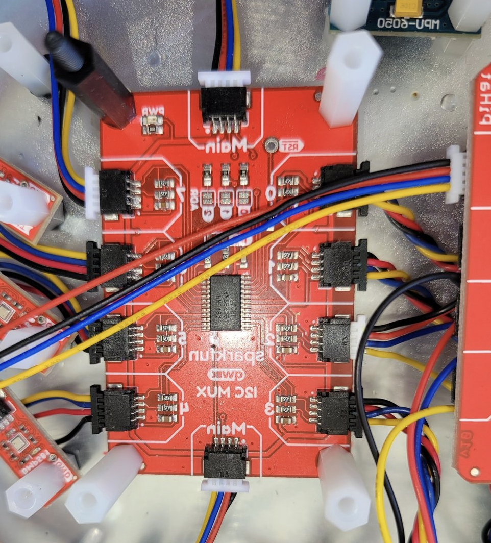
Multiplexer arrays
For the patent prototype, we used TCA9548A 8-channel I2C multiplexers. Each mux channel is an electrically isolated I2C bus, so sensors on different channels can share the same address:
                          ┌─── ch 0 ─── BMP280 (0x76) + BMP280 (0x77)
  Pi ── I2C ── TCA9548A ──┼─── ch 1 ─── BMP280 (0x76) + BMP280 (0x77)
               (addr 0x70) ├─── ch 2 ─── BMP280 (0x76) + BMP280 (0x77)
                          └─── ...         (up to 16 sensors per mux)
A Raspberry Pi at each location ran a Rust application on Linux that cycled through mux channels, read calibrated pressure/temperature data from every sensor, and logged the raw values. A separate PC-based Rust application pulled the log files for analysis, producing plots and spreadsheets.
What We Learned: BMP280 → BMP581
The BMP280 worked for the initial proof-of-concept, but we hit its limits. The sensor’s resolution wasn’t granular enough for the pressure differentials we needed to measure. The BMP581—Bosch’s newer generation—offers significantly better resolution and noise characteristics.
We also changed the architecture. Instead of running I2C extenders to reach distant sensor locations from a single controller, we gave each location its own Raspberry Pi with its own mux and BMP581 sensor array. The Pi boards communicate over gigabit LAN, which is simpler, more reliable, and eliminates the signal integrity issues that come with long I2C runs.
Location A:  Pi ── I2C ── TCA9548A ── BMP581s ──┐
                                                  ├── Gigabit LAN
Location B:  Pi ── I2C ── TCA9548A ── BMP581s ──┘
                                                  │
                                        Analysis PC (Rust)
Using the Driver
Basic usage with a single sensor:
use bmp280_ehal::BMP280;

let mut bmp = BMP280::new(i2c)?;
let temp = bmp.temp(0x76);     // Celsius
let pres = bmp.pressure(0x76); // Pascals
Two sensors on one bus:
let mut bmp = BMP280::new(i2c)?;
bmp.read_calibration(0x77);

let delta_p = bmp.pressure(0x76) - bmp.pressure(0x77);
With a multiplexer:
fn select_channel<I2C, E>(i2c: &mut I2C, ch: u8) -> Result<(), E>
where I2C: embedded_hal::blocking::i2c::Write<Error = E>
{
    i2c.write(0x70, &[1 << ch])
}
See the multi-sensor documentation for shared-bus patterns and cascaded mux topologies.
Fun Fact: Some of the Raspberry Pi boards with I2C multiplexers and BMP581 sensor arrays were submerged in diving bell-like enclosures with low power and LAN cables tethered.
References
Reference Link BMP280 datasheet Bosch Sensortec (PDF) BMP581 product page Bosch Sensortec MIKROE Pressure 21 Click mikroe.com I2C Multiplexer (TCA9548A) SparkFun I2C Mux US Patent 12,188,836 B1 Google Patents Multi-sensor docs GitHub Part 1 of the Embedded series. View all parts | Next: Part 2 →
Comments or questions? SW Lab Discord or YouTube @SoftwareWrighter.
-
584 words • 3 min read • Abstract
AI Tools #1: XSkill --- A Memory Layer for Multimodal Agents

Resource Link Paper arXiv 2603.12056 Project XSkill Project Page Code GitHub (MIT) Video XSkill: Memory Layer 
Comments Discord The Problem: Isolated Episodes
Multimodal agents solve complex visual and tool-heavy tasks, but each run starts from scratch. An agent might figure out a multi-step workflow for extracting color data from an image—only to lose that knowledge when the next task begins. Useful lessons evaporate between sessions.
Two Kinds of Memory
XSkill introduces a dual-memory architecture that separates strategic knowledge from tactical knowledge:
Skills are structured Markdown documents containing workflows and tool templates for a class of tasks. A skill says: here is the overall approach for this kind of problem.
Experiences are smaller tactical lessons with triggering conditions, recommended actions, and failure notes. An experience says: when this specific pattern appears, use this tactic instead of guessing.
That split matters. Ablation analysis shows that removing either type hurts performance—skills alone aren’t enough, and experiences alone aren’t enough.
Two-Phase Framework
The framework operates in a loop:
Phase 1 — Accumulation. After completing rollout batches, the agent reviews past trajectories through visually-grounded summarization, cross-rollout critique, and hierarchical consolidation. This produces skill documents and experience items stored in persistent banks.
Phase 2 — Inference. Given a new task, the agent decomposes it, retrieves relevant skills and experiences via semantic search, adapts them to the current visual context, and injects them into the system prompt.
The key claim: agents improve through memory accumulation and retrieval, not parameter updates. No fine-tuning required.
Results
Evaluated across five benchmarks spanning visual tool use (VisualToolBench, TIR-Bench), multimodal search (MMSearch-Plus, MMBrowseComp), and comprehensive agent tasks (AgentVista):
Backbone Avg@4 Pass@4 Gemini-3-Flash + XSkill 40.34 58.95 Gemini-2.5-Pro + XSkill 28.63 46.38 o4-mini + XSkill 23.72 39.07 GPT-4o-mini + XSkill 23.19 38.90 Average gains of 2.6 to 6.7 points over baselines (Agent Workflow Memory, Dynamic CheatSheet, Agent-KB). Performance consistently improves as rollout count increases from 1 to 4.
Practical impact: syntax errors drop from 20.3% to 11.4% with skills, and tool name errors fall from 2.85% to 0.32%.
Concrete Example
A visual task requires identifying the color of a region behind specific text in an image. Without memory, the agent guesses. With XSkill, it retrieves a structured workflow: locate the text, isolate the region, sample pixels via code interpreter, and infer the color from actual data. Code interpreter usage increases from 66.6% to 77.0% on VisualToolBench—the agent learns to measure instead of guess.
Why This Matters
XSkill sits at the intersection of agents, tools, multimodal reasoning, and continual improvement. The practical takeaway isn’t just that memory helps—it’s that different kinds of memory help in different ways. Strategic workflows and situational tactics serve complementary roles.
Not a bigger model. A smarter memory layer.
References
Reference Link XSkill paper arXiv 2603.12056 Project page xskill-agent.github.io GitHub repo (MIT) XSkill-Agent/XSkill Part 1 of the AI Tools series. View all parts | Next: Part 2 →
Comments or questions? SW Lab Discord or YouTube @SoftwareWrighter.
-
823 words • 5 min read • Abstract
ML Frontier #02: In-Context Reinforcement Learning

Second ML Frontier episode. This one covers In-Context Reinforcement Learning—how transformers learn decision policies from trajectory examples in the prompt, without weight updates.
Resource Link Papers 5 papers covered Video ML Frontier 2: ICRL 
Related Saw #2: agentrail-rs — practical ICRL application Comments Discord What is In-Context Reinforcement Learning?
The model observes sequences of states, actions, and rewards stored in the prompt. Instead of updating weights through gradient descent, the transformer approximates a policy from those trajectory examples.
Think of it like learning to cook by reading a journal of recipes that worked—and ones that didn’t—with notes on what went wrong.
Why Does This Matter?
AI agents often lose procedural knowledge when context is truncated between sessions. They know the goal but forget which API to call, which flags to use, which client library to reference, or how to validate output.
The traditional approach—writing instructions in markdown files—isn’t reliable. Agents ignore rules even when they’re present. ICRL offers a different path: instead of telling the agent what to do, show it what worked and what didn’t, with reward signals attached.
By embedding successful execution traces in the prompt, agents can reuse proven approaches instead of improvising from scratch.
Research Evidence
Decision Transformer (Chen et al., 2021)
Paper: arXiv 2106.01345
In brief: The paper that started it all. Instead of training an RL agent with value functions and policy gradients, just frame the problem as sequence prediction. Feed the transformer trajectories of (return-to-go, state, action) and let it predict the next action conditioned on the desired return. The transformer learns a policy by modeling sequences—no Bellman equations needed.
Why it matters: Reframed RL as something transformers already do well: sequence modeling.
Transformers Learn TD Methods (Wang et al., ICLR 2025)
Paper: arXiv 2405.13861
In brief: This paper shows that transformers don’t just pattern-match on trajectories—they actually approximate temporal-difference (TD) learning algorithms during the forward pass. The model internally implements something resembling TD updates, without being explicitly trained to do so.
Why it matters: Transformers aren’t just memorizing trajectories. They’re learning the underlying RL algorithm in-context.
OmniRL (2025)
Paper: arXiv 2502.02869
In brief: OmniRL proposes a transformer architecture that emulates actor-critic RL in-context, improving decision quality across multiple tasks. Rather than specializing in one environment, the model generalizes its in-context RL capabilities across diverse settings.
Why it matters: ICRL isn’t limited to one task—it scales across environments.
Reflexion (Shinn et al., NeurIPS 2023)
Paper: arXiv 2303.11366
In brief: Reflexion takes a different angle: instead of embedding raw trajectories, the agent generates verbal reflections on its failures and successes. These self-critiques are stored and injected into future prompts. The agent learns from its own written analysis of what went wrong.
Why it matters: Shows that trajectory-based learning doesn’t require structured (state, action, reward) tuples—natural language reflections work too.
Voyager (Wang et al., 2023)
Paper: arXiv 2305.16291
In brief: An open-ended Minecraft agent that builds a skill library from successful code executions. When Voyager solves a task, it stores the working code as a reusable skill. Future tasks can retrieve and compose these skills. The agent explores, learns, and accumulates capabilities without any weight updates.
Why it matters: Demonstrates ICRL at scale—an agent that gets better over time by accumulating proven solutions.
Papers
Date Paper Link Jun 2021 Decision Transformer: RL via Sequence Modeling arXiv 2106.01345 Mar 2023 Reflexion: Language Agents with Verbal Reinforcement Learning arXiv 2303.11366 May 2023 Voyager: Open-Ended Embodied Agent with LLMs arXiv 2305.16291 May 2024 Transformers Learn TD Methods for In-Context RL arXiv 2405.13861 Feb 2025 OmniRL: In-Context RL Across Multiple Tasks arXiv 2502.02869 Practical Application: agentrail-rs
This isn’t just theory. I’m building agentrail-rs to apply ICRL to AI coding agents used for non-coding tasks—TTS generation, video compositing, file manipulation. The tool records trajectories (state, action, result, reward) and injects successful examples into future agent prompts. Early days, but the research says this should work.
See Saw #2: agentrail-rs for more on the engineering side.
Key Takeaways
Concept One-liner ICRL Learn RL policies from trajectory examples in the prompt No Weight Updates The transformer adapts during inference, not training TD in the Forward Pass Transformers approximate RL algorithms internally Verbal Reflection Natural language self-critique works as trajectory data Skill Libraries Accumulate proven solutions for reuse across sessions
In-Context RL turns agents from amnesiacs into learners. Follow for more ML Frontier episodes exploring research at the edge.
Part 2 of the Machine Learning Frontier series. View all parts | Next: Part 3 →
Comments or questions? SW Lab Discord or YouTube @SoftwareWrighter.
-
1876 words • 10 min read • Abstract
Saw #2: reg-rs, avoid-compaction, and agentrail-rs

Welcome back to the Sharpen the Saw series, where I maintain existing tools, vibe-code new ones, and try new approaches to development workflows. Three tools, one pattern: each one hit a ceiling that required rethinking how it stores and shares information. This week covers reg-rs migrating from binary to text-based test definitions, avoid-compaction structuring multi-session AI agent workflows, and agentrail-rs adding reinforcement learning from an agent’s own success history.
Resource Link Repos sw-cli-tools/reg-rs, softwarewrighter/avoid-compaction, sw-vibe-coding/agentrail-rs Video Sharpening 3 Rust Dev Tools References Links and Resources Comments Discord reg-rs: Three Improvements to Regression Testing
reg-rs captures command output as golden baselines and flags regressions on re-run. This round of sharpening addressed three friction points: clunky commands, opaque binary storage, and noisy output.
Shell Aliases
The full command syntax (
reg-rs run -p my_test -v) gets old fast. Shell aliases insource-rg.shcut it to 4 characters with tab completion in zsh and bash:Alias Action Example rnrgRun tests rnrg my_test -vadrgCreate test adrg my_test 'echo hi'lsrgList tests lsrgshrgShow details shrg my_test -vvuprgRebase baselines uprg my_testrsrgReset results rsrg my_testrmrgRemove test rmrg old_testmgrgMigrate .tdb to .rgt mgrgstrgStatus dashboard strgMuscle memory builds fast.
hlrgprints the full cheat sheet with examples.Git-Friendly .rgt Format
The legacy
.tdbformat stored tests in SQLite binary files.git diffshowed noise, merge conflicts were unresolvable, and new developers needed setup scripts. Regression tests are documentation—they define what your CLI actually does—so hiding them in binary blobs defeated the purpose.The new
.rgtformat splits each test across git-tracked text files:File Contents Tracked? test.rgtTOML spec (command, timeout, preprocessing) Yes test.outExpected stdout baseline Yes test.errExpected stderr (only if non-empty) Yes test.tdbRuntime cache No (gitignored) A test definition reads like documentation:
command = "myapp --version"
timeout = 10
exit_code = 0
desc = "Version string format check"
preprocess = "jq --sort-keys"
diff_mode = "json"
reg-rs createnow writes.rgtdirectly—no intermediate.tdbstep. Existing tests migrate withmgrg. PR reviewers see exactly what changed and why,git cloneinherits every test, and merge conflicts resolve with standard tools.Output Verbosity Controls
Previously, running tests dumped SQL debug info and full diffs regardless of context. Now output scales to what you need:
Flag Output (none) Summary line: 3 passed, 1 failed (of 4 total)-v+ failure details (diff counts per test) -vv+ full diff output -qNothing—exit code only Exit codes are now meaningful too:
0for all pass,1for regressions detected,2for errors. This makes reg-rs usable in CI pipelines where you check$?rather than parse output.Sharpen the Saw — Habit 7 from Stephen Covey’s The 7 Habits of Highly Effective People is about preserving and enhancing your greatest asset: yourself and your tools. In software, that means taking time to fix accumulated friction, update dependencies, and learn new frameworks—even when shipping features feels more urgent. The payoff compounds: every hour spent sharpening saves many more down the line.
avoid-compaction: Structured Multi-Session Agent Workflows
avoid-compaction solves a problem anyone using AI coding agents hits eventually: context death. Long conversations get automatically compacted—the system summarizes older messages to make room for new ones, losing decisions, constraints, and procedural knowledge along the way.
The Insight
Rather than fighting compaction with longer context windows, avoid-compaction embraces frequent restarts as a feature. Each restart gives the agent a full, fresh context window. The trick is making handoffs explicit and structured so nothing is lost between sessions.
The Saga/Step Model
Work is organized into sagas (projects) composed of steps (focused units of work):
.avoid-compaction/
  saga.toml                    # name, status, current step
  plan.md                      # evolving project plan
  planned-steps.md             # upcoming steps preview
  steps/001-add-routes/
    step.toml                  # status, description, context files
    prompt.md                  # what the agent was told to do
    summary.md                 # what the agent actually did
  steps/002-add-tests/
    ...
Each session follows the same loop:
- New Claude session starts with fresh context
- Agent runs
nextto see the current step’s prompt and context - Agent does the work
- Agent runs
completewith a summary and next-step definition - User restarts Claude
- Next session picks up exactly where the last left off
Why This Matters
The difference is reliability. Without structured handoffs, session 4 of a complex feature often forgets constraints from session 1. The agent improvises, makes contradictory decisions, or redoes work. With avoid-compaction:
- Every session starts with full context for its specific task
- Summaries accumulate so later sessions can reference earlier decisions
- The plan evolves as work reveals new insights
- Nothing is lost to compaction—it’s all in the filesystem
Current Improvements
The tool is going through a refactoring sequence to meet code quality standards:
- Merging small command modules into larger, cohesive modules
- Extracting shared display logic into reusable formatters
- Workspace conversion to split concerns across crates
- Session crate extraction for reusable JSONL handling
Each spike is low-to-medium risk, guided by the principle that smaller modules with clear responsibilities are easier to test, review, and extend.
agentrail-rs: Learning from Success
agentrail-rs is the evolution of avoid-compaction, adding a critical capability: In-Context Reinforcement Learning (ICRL). Where avoid-compaction structures handoffs, agentrail-rs teaches agents from their own history.
The 75% Problem
I use AI coding agents for more than coding—TTS audio generation, video compositing, file manipulation, and other multi-step production tasks. In practice, agents succeed about 75% of the time on these workflows. The failures aren’t random—they’re procedural: the agent forgets which API to call, which flags to use, which client library to reference, or how to validate output.
The traditional approach—writing instructions in markdown files like
AGENTS.mdorCLAUDE.md—isn’t reliable. Even when rules, instructions, and prohibitions are present, agents often ignore them. Claude, when called out, will say “You’re right, I should have done that”—and a few moments later make the same kind of mistake. Bigger prompts and more examples hit diminishing returns. The agent needs to learn from reward-based examples—both good and bad—delivered in-context, not static documentation it may or may not follow. That’s the core idea behind ICRL: show the agent what worked, what didn’t, and let the rewards guide its next attempt.How ICRL Works
After each step, agentrail-rs records a trajectory:
state → action → result → rewardSuccessful trajectories are stored at
.agentrail/trajectories/{task_type}/run_NNN.json. When the agent hits the same task type in a new session, the CLI retrieves the top N successful trajectories and injects them into the prompt: “Here’s how you succeeded at this before.”The agent reads its own success patterns and self-corrects—no weight updates, no fine-tuning, no training pipeline. Just examples from its own history, delivered in context.
Four Step Types
agentrail-rs distinguishes what needs an agent from what doesn’t:
Step Type Who Executes Example Meta Agent Prepare handoff packets with success examples Production Agent Execute semantic work using prepared context Deterministic Machine Run TTS generation, video composition (no agent needed) Validation Machine Check outputs, record rewards for ICRL Deterministic steps can’t fail due to agent forgetfulness—they’re hard-specified. Validation steps create the reward signals that make ICRL work.
Architecture
The project is structured as a five-crate Cargo workspace:
Crate Purpose Status agentrail-coreDomain model, trajectories, handoff packets Complete agentrail-storePersistence (saga, step, trajectory, session) Complete agentrail-cliCLI commands Stub agentrail-execDeterministic job executors Stub agentrail-validateOutput validators Stub The core and store crates are done. The next phase wires up the CLI, then deterministic execution, then the full ICRL retrieval and injection loop.
The Expected Payoff
Once the trajectory system is live (I just started vibe-coding it today), agents working on repetitive task types should see reliability climb from ~75% toward deterministic. Each success makes the next attempt more likely to succeed, without any manual intervention. The goal is a self-improving loop: agents learn their own procedures through experience.
Three Problems, Three Approaches
These projects aren’t related by a common architecture or shared abstraction. They’re related because each one solves a different productivity problem I keep hitting:
- reg-rs catches regressions that slip in whenever a feature is added or a fix applied—the kind of silent breakage that unit tests don’t cover because they test behavior, not actual output.
- avoid-compaction is a direct reaction to Claude Code auto-compacting multiple times per day, with noticeable performance degradation after each compaction. Structured restarts with explicit handoffs beat a slowly decaying context window.
- agentrail-rs tackles the opposite problem: not forgetting, but improvising. LLMs are probabilistic, and Claude keeps trying new (failing) approaches to routine tasks instead of sticking with the proven-working ones it has used and documented before. ICRL feeds successful trajectories back into context so the agent repeats what works.
Different problems, different solutions, same goal: spend less time fighting tools and more time building.
References
Resource Link reg-rs github.com/sw-cli-tools/reg-rs avoid-compaction github.com/softwarewrighter/avoid-compaction agentrail-rs github.com/sw-vibe-coding/agentrail-rs Decision Transformer Chen et al., 2021 — framing RL as sequence modeling Transformers Learn TD Methods Wang et al., ICLR 2025 — transformers simulate temporal-difference learning in-context OmniRL 2025 — transformer architecture emulating actor-critic RL in-context Reflexion Shinn et al., NeurIPS 2023 — verbal self-reflection for agent improvement Voyager Wang et al., 2023 — open-ended learning agent with skill library “Sharpen the Saw” The 7 Habits of Highly Effective People (Stephen Covey)
Habit 7: Sharpen the Saw. Spend less time fighting tools, more time building.
Part 2 of the Sharpen the Saw Sundays series. View all parts | Next: Part 3 →
Comments or questions? SW Lab Discord or YouTube @SoftwareWrighter.
-
2797 words • 14 min read • Abstract
Rabbit-hole #1: Poor Man's Rust-to-Unsupported-ISA Translator

Resource Link Live Demo COR24 Assembly Emulator Source GitHub MakerLisp makerlisp.com (COR24 creators) Disclaimer Proof of concept only Comments Discord
The Problem
COR24 is a 24-bit RISC soft CPU designed by MakerLisp for FPGAs. It has 3 general-purpose registers, a 24-bit address space, and runs at 101 MHz on inexpensive Lattice FPGAs. It’s MIT-licensed, well-documented, and has real hardware you can buy.
But LLVM doesn’t have a COR24 backend. Neither does GCC. Writing a full compiler backend could take a lot more effort. We need another way in.
The Trick: Borrow a Target
rustcsupports MSP430, a 16-bit TI microcontroller, via LLVM’s MSP430 backend. It’s a nightly-only target (msp430-none-elf), but it works. The key insight: MSP430’s instruction set is close enough to COR24 that a translator can bridge the gap.The full pipeline:
Rust Source (.rs)
     ↓  rustc --target msp430-none-elf --emit asm
MSP430 Assembly (.msp430.s)
     ↓  msp430-to-cor24 translator
COR24 Assembly (.cor24.s)
     ↓  COR24 assembler
Machine Code → COR24 Emulator (or real FPGA hardware)
No custom compiler. No modified LLVM. Just Rust’s nightly toolchain and a ~1,800-line translator written in Rust. This is a proof-of-concept—an educational demo, not a production tool for real COR24 hardware.
Disclaimer
This is a proof-of-concept and educational demo. The MSP430-to-COR24 translator is not intended for production use on real COR24 hardware. It demonstrates that the approach is feasible, not that it’s complete or reliable. If you’re building something real on COR24, use the native assembler and toolchain from MakerLisp.
Level 1: The Compiler Optimizes Away Your Code
Let’s start simple. Three numbers, one add:
#![no_std]

const RESULT_ADDR: u16 = 0x0100;

#[inline(never)]
#[no_mangle]
pub fn demo_add() -> u16 {
    let a: u16 = 100;
    let b: u16 = 200;
    let c: u16 = 42;
    a + b + c  // Returns 342
}

#[no_mangle]
pub unsafe fn start() -> ! {
    let result = demo_add();
    core::ptr::write_volatile(RESULT_ADDR as *mut u16, result);
    loop {}
}
Compile to MSP430 and the rabbit hole opens immediately. Here’s what
rustcemits fordemo_add:demo_add: mov #342, r12 retTwo instructions. LLVM constant-folded
100 + 200 + 42into342at compile time. The addition doesn’t exist in the output—the compiler proved the answer is always the same and replaced the computation with a constant load.The translator converts this to COR24:
demo_add:
    la      r0, 0x000156    ; load 342 (24-bit)
    jmp     (r1)            ; return via r1
Run it in the emulator (
scripts/demo-add.sh):Executed 3 instructions CPU halted (self-branch detected) === Registers === r0: 0x000156 ( 342)Two instructions in
demo_add, three total to reach halt. The “add” demo that doesn’t add.
Level 1.5: More Variables Than Registers
What happens when Rust needs more live variables than COR24 has registers? MSP430 has 12 general-purpose registers. COR24 has 3. The translator has to spill the extras to the stack.
The
accumulatefunction keeps 5 values alive simultaneously:#[inline(never)] #[no_mangle] pub unsafe fn accumulate(seed: u16) -> u16 { let a = seed + 1; let b = a + seed; let c = b + a; let d = c + b; let e = d + c; let result = a ^ b ^ c ^ d ^ e; mem_write(RESULT_ADDR, result as u8); uart_putc(a); uart_putc(b); uart_putc(c); uart_putc(d); uart_putc(e); loop {} }The MSP430 assembly uses registers
r6throughr10—five registers that don’t exist on COR24:accumulate: push r6 push r7 push r8 push r9 push r10 ; save 5 callee-saved registers mov r12, r10 ; seed mov r10, r6 inc r6 ; a = seed + 1 add r6, r10 ; b = a + seed mov r10, r9 add r6, r9 ; c = b + a ...The translator maps these to frame-pointer-relative stack slots, each 3 bytes (one COR24 word). Where MSP430 writes
mov r10, r6, COR24 must load from one spill slot, operate, and store to another:accumulate: sw r0, 30(fp) ; spill seed (r10 → offset 30) lw r0, 6(fp) ; save spill slot for r6 push r0 ... lw r0, 18(fp) ; load r10 (seed) sw r0, 6(fp) ; copy to r6 slot lw r0, 6(fp) ; load r6 add r0, 1 ; a = seed + 1 sw r0, 6(fp) ; store r6 back ... la r0, 0xFF0000 ; RESULT_ADDR ; call mmio_write push r1 la r2, mmio_write jal r1, (r2) ; jal saves return addr in r1 pop r1It’s verbose—the COR24 output is much longer than the MSP430 input. But it’s correct. The emulator confirms the computation with 148 instructions and the XOR result stored to memory at
0x0100.
Level 2: The Compiler Writes Your Destructor
Rust’s Drop trait guarantees cleanup when a value goes out of scope. Does that work on a CPU with no OS, no allocator, no runtime?
pub struct Guard { addr: u16 }

impl Guard {
    #[inline(never)]
    #[no_mangle]
    pub fn guard_new(addr: u16) -> Guard {
        unsafe { mem_write(addr, 1); }  // mark: alive
        Guard { addr }
    }
}

impl Drop for Guard {
    #[inline(never)]
    fn drop(&mut self) {
        unsafe { mem_write(self.addr, 0); }  // mark: gone
    }
}

#[no_mangle]
pub unsafe fn start() -> ! {
    {
        let _g = Guard::guard_new(STATUS_ADDR);
        // STATUS_ADDR = 1 (guard is alive)
    }
    // STATUS_ADDR = 0 (compiler called drop here)

    mem_write(STATUS_ADDR, 0xFF);  // proof we continued
    loop {}
}
Look at the MSP430 assembly for
start—the compiler inserted the drop call:start: sub #2, r1 ; allocate stack space mov #256, r12 ; STATUS_ADDR call #guard_new ; create guard → writes 1 mov #256, 0(r1) ; store Guard on stack mov r1, r12 ; pass &Guard to drop call #<Guard::drop> ; compiler-inserted! → writes 0 mov #256, r12 mov #255, r13 call #mem_write ; writes 0xFF .LBB4_1: jmp .LBB4_1 ; haltThe
call #<Guard::drop>on line 6 is the compiler honoring the Drop contract. You didn’t write that call—rustcdid. Memory atSTATUS_ADDRgoes:0 → 1 → 0 → 0xFF, proving the destructor ran at the right moment.The translated COR24 assembly preserves this structure—each
callbecomes ajal(jump-and-link), which saves the return address inr1:start: sub sp, 3 ; allocate stack space la r0, 0x000100 ; STATUS_ADDR ; call guard_new push r1 la r2, guard_new jal r1, (r2) ; create guard → writes 1 pop r1 ... ; call <Guard::drop> ; compiler-inserted! push r1 la r2, <Guard::drop> jal r1, (r2) ; → writes 0 pop r1RAII works on bare metal, on an architecture the Rust compiler has never heard of.
Level 3: Interrupts via
asm!PassthroughHere’s where it gets interesting. COR24’s interrupt mechanism uses hardware registers that MSP430 doesn’t have:
- iv: Interrupt vector—CPU jumps here when an interrupt fires
- ir: Interrupt return—saved PC to return to after the ISR
jmp (ir): Return from interrupt
There’s no MSP430 equivalent—the LLVM backend has no concept of these registers. But Rust’s
asm!macro combined with the translator’s passthrough mechanism can handle it.The
demo_echo_v2example splits the problem: application logic in pure Rust, interrupt plumbing inasm!passthrough:#![feature(asm_experimental_arch)] /// Application logic --- pure Rust, compiled normally #[inline(never)] #[no_mangle] pub fn to_upper(ch: u16) -> u16 { if ch >= 0x61 && ch <= 0x7A { ch & 0xDF // clear bit 5 } else { ch } } #[inline(never)] #[no_mangle] pub unsafe fn handle_rx() { let ch = mmio_read(UART_DATA); if ch == 0x21 { // '!' mmio_write(HALT_FLAG, 1); } else { uart_putc(to_upper(ch)); } }The ISR wrapper uses
asm!with a@cor24:prefix that the translator passes through verbatim:#[no_mangle] pub unsafe fn isr_handler() { // Save COR24 state (asm! --- no Rust equivalent) core::arch::asm!( "; @cor24: push r0", "; @cor24: push r1", "; @cor24: push r2", "; @cor24: mov r2, c", // save condition flag "; @cor24: push r2", ); handle_rx(); // ← pure Rust, compiled through the pipeline // Restore state and return from interrupt core::arch::asm!( "; @cor24: pop r2", "; @cor24: clu z, r2", // restore condition flag "; @cor24: pop r2", "; @cor24: pop r1", "; @cor24: pop r0", "; @cor24: jmp (ir)", // return from interrupt options(noreturn) ); }The
"; @cor24: ..."lines look like MSP430 comments (sorustcignores them), but the translator recognizes the prefix and emits them as real COR24 instructions. In the final COR24 assembly:isr_handler: push r0 push r1 push r2 mov r2, c ; save condition flag push r2 ; call handle_rx ← compiled Rust push r1 la r2, handle_rx jal r1, (r2) ; jal saves return addr in r1 pop r1 pop r2 clu z, r2 ; restore condition flag pop r2 pop r1 pop r0 jmp (ir) ← hardware interrupt returnThe
startfunction sets up the interrupt vector and enables UART reception:core::arch::asm!( "; @cor24: la r0, isr_handler", "; @cor24: mov iv, r0", // iv = interrupt vector register "; @cor24: lc r0, 1", "; @cor24: la r1, 0xFF0010", // UART interrupt enable register "; @cor24: sb r0, 0(r1)", // enable UART RX interrupt );Type a letter, the hardware fires an interrupt, the ISR saves registers, calls
handle_rx(compiled Rust), converts to uppercase, echoes it via UART, restores registers, and returns. The boundary between Rust and hardware is exactly where you’d expect it.
What the Translator Actually Does
The
msp430-to-cor24translator (~1,800 lines of Rust) handles the mechanical differences:Concern MSP430 COR24 Translation Word size 16-bit 24-bit Stack slots: 2 bytes → 3 bytes Registers r12-r14 (args) r0-r2 (args) Direct mapping Spilled regs r4-r11 (MSP430) None (3 GPRs only) Frame-pointer relative loads/stores I/O addresses 16-bit (0xFF00) 24-bit (0xFF0000) Address remapping Call convention call #func/retjal r1, (r2)/jmp (r1)Uses COR24’s jump-and-link Tail calls call+retpatternjmp (r2)Direct jump, no link Entry point Section order Reset vector at addr 0 la r0, start+jmp (r0)COR24’s calling convention centers on the
jal(jump-and-link) instruction.jal r1, (r2)jumps to the address inr2and saves the return address inr1. The callee returns withjmp (r1). Since the translator re-usesr1for the return address, it saves and restoresr1around each call withpush r1/pop r1. COR24’s native C compiler convention uses a standard prologue (push fp; push r2; push r1; mov fp,sp) and passes arguments on the stack—the translator doesn’t follow that full protocol, but it does use the samejal/jmp (r1)mechanism for call and return.The entry point handling is worth noting.
rustcemits functions in alphabetical section order, so the panic handler often lands at address 0. Every demo uses a#[no_mangle] pub unsafe fn start() -> !as its entry point—a convention I chose for this project. The translator looks for astartlabel and emits a reset vector prologue (la r0, start+jmp (r0)at address 0), mimicking how real microcontrollers boot. This isn’t a Rust or MSP430 convention; it’s a project-level rule that keeps the translator simple and every demo consistent.
Try It Yourself
# Prerequisites
rustup toolchain install nightly
rustup target add msp430-none-elf --toolchain nightly

# Clone and build
git clone https://github.com/sw-embed/cor24-rs.git
cd cor24-rs/rust-to-cor24

# Run the add demo (full pipeline)
bash scripts/demo-add.sh

# Run the UART hello demo
bash scripts/demo-uart-hello.sh

# Or compile any demo project
cargo run --bin msp430-to-cor24 -- --compile demos/demo_drop
Each demo script traces the full pipeline: Rust source → MSP430 assembly → COR24 assembly → emulator output with register dumps.
Key Takeaways
-
You don’t need a compiler backend to target a new architecture. If a similar-enough target exists, a translator can bridge the gap.
-
The Rust compiler is surprisingly good at bare-metal code. Constant folding, dead code elimination, and Drop all work correctly even when the output gets re-targeted to an architecture LLVM has never seen.
-
asm!passthrough is the escape hatch. Hardware-specific operations (interrupt setup, condition flag save/restore) bypass the translation layer entirely using comment-prefix conventions. -
The pipeline is auditable. Every intermediate artifact (
.msp430.s,.cor24.s, register dumps) is human-readable. You can trace any behavior from source to silicon.
The rabbit hole goes deeper. Next time: what happens when the 16-bit intermediate can’t express a 24-bit value.
Part 1 of the Down the Rabbit-Hole series. View all parts | Next: Part 2 →
Comments or questions? SW Lab Discord or YouTube @SoftwareWrighter.
-
736 words • 4 min read • Abstract
ML Frontier #01: Neural Collapse

First Machine Learning Mondays post. ML Frontier explores cutting-edge research in machine learning.
Resource Link Papers 5 papers covered Video ML Frontier #01: Neural Collapse 
Comments Discord What is Neural Collapse?
During the final phase of training, deep network representations converge to a specific geometric pattern. Class means become equidistant and form a symmetric simplex structure in the feature space.
Think of it like points arranging themselves at equal distances on a sphere.
Why Does This Happen?
When networks are trained past zero training error, representations continue simplifying. The network finds the most symmetric way to separate classes, forming equal angles between all class centers.
This isn’t random—it’s mathematically optimal.
2024-2025 Breakthroughs
Recent research proves neural collapse is globally optimal in deep transformers and ResNets with regularization. As depth increases, the network provably converges to this collapsed geometry.
This changes how we think about deep learning. Collapse explains why overparameterized networks generalize well. It also guides continual learning, where progressive collapse prevents catastrophic forgetting.
Papers
Date Paper Link Sep 2024 Beyond Unconstrained Features: Neural Collapse for Shallow Networks arXiv 2409.01832 Oct 2024 Wide Neural Networks with Weight Decay Provably Exhibit Neural Collapse arXiv 2410.04887 Jan 2025 Neural Collapse Beyond the Unconstrained Features Model arXiv 2501.19104 May 2025 Rethinking Continual Learning with Progressive Neural Collapse arXiv 2505.24254 May 2025 Neural Collapse is Globally Optimal in Deep Regularized ResNets and Transformers arXiv 2505.15239 Paper Summaries
Beyond Unconstrained Features (Sep 2024)
Paper: Hong & Ling
In brief: Most neural collapse theory assumes you can put class markers anywhere you want—like sticking Post-it notes anywhere on a wall. But real shallow networks have limits. This paper shows neural collapse still emerges even in small networks with real data constraints, not just idealized deep networks.
Why it matters: Neural collapse isn’t just a “big model” phenomenon—it happens in smaller, practical architectures too.
Wide Networks with Weight Decay (Oct 2024)
Paper: Jacot, Súkeník, Wang & Mondelli
In brief: If you train a wide neural network with weight decay (a common regularization trick), this paper proves the network will exhibit neural collapse. It’s the first proof that end-to-end training (not just theory) leads to collapse.
Why it matters: Weight decay isn’t just preventing overfitting—it’s actively pushing the network toward optimal geometry.
Beyond the Unconstrained Features Model (Jan 2025)
Paper: arXiv 2501.19104
In brief: The “unconstrained features model” assumes networks can place representations anywhere. Real networks have architectural constraints. This paper extends neural collapse theory to realistic settings where the architecture limits what’s possible.
Why it matters: The theory holds up in real-world conditions, not just toy examples.
Progressive Neural Collapse for Continual Learning (May 2025)
Paper: arXiv 2505.24254
In brief: When you teach a network new things, it often forgets old things (catastrophic forgetting). This paper uses neural collapse to fix that: by carefully managing how class representations “collapse” over time, the network can keep learning new tasks without losing old knowledge.
Why it matters: Neural collapse isn’t just a curiosity—it’s a tool for building better learning systems.
Globally Optimal in Transformers and ResNets (May 2025)
Paper: Súkeník et al.
In brief: Imagine you have a box of crayons and need to organize them so each color is as far from every other color as possible. This paper proves that deep neural networks automatically find the best possible arrangement—not just a good one, but the mathematically perfect one. And this happens in both transformers (like GPT) and ResNets (like image classifiers).
Why it matters: It’s not a coincidence that networks learn this way. It’s provably optimal.
Key Takeaways
Concept One-liner Neural Collapse Class representations converge to symmetric simplex geometry Why It Happens Training past zero error simplifies representations maximally Optimal Geometry Provably the best configuration in deep networks Practical Impact Explains generalization and enables continual learning
Neural collapse reveals the hidden geometry of learning. Follow for more ML Frontier episodes exploring cutting-edge research.
Part 1 of the Machine Learning Frontier series. View all parts | Next: Part 2 →
Comments or questions? SW Lab Discord or YouTube @SoftwareWrighter.
-
2775 words • 14 min read • Abstract
Saw #1: pjmai-rs, Rig, and langchain-rust

Three tools, one theme: sharpening the foundation. This week covers pjmai-rs bug fixes and new features, plus a first look at two Rust frameworks for building LLM-powered applications—Rig and langchain-rust.
Resource Link Repos sw-cli-tools/pjmai-rs, try-rig, try-langchain-rust Video Explainer References Links and Resources Comments Discord pjmai-rs: Fixing the Foundation
Before adding AI features to any tool, you need a solid foundation. Since the last update, pjmai-rs received critical fixes and practical new features.
The Rust 2024 Edition Bug
Upgrading to Rust edition 2024 broke project removal silently. The
IndexMap::remove()method changed semantics—it now preserves insertion order differently. The fix:// Rust 2024 broke this - projects.remove(name) // shift_remove maintains expected behavior + projects.shift_remove(name)A one-line fix, but the kind that silently corrupts data if you miss it. The 2024 edition migration guide mentions this change, but it’s easy to overlook in a large codebase.
Shell Integration Improvements
- Help flags: All aliases (
chpj,hypj,stpj, etc.) now properly pass--helpthrough - After-help messages: Every subcommand shows examples and related commands
- Version matching:
--versionoutput now matchesCargo.toml - Argument validation: Better error messages for invalid flag combinations
New Capabilities
Feature Command What It Does Stack navigation stpjPush/pop project context with visibility History tracking hypjRevisit recently-visited projects by number Fuzzy completion chpj <TAB>Prefix > segment > substring, sorted by recency Environment config evpjPer-project env vars with auto-detection (Python, Node, Rust) Bulk operations rmpj --allBatch management with confirmation Subdirectory nav chpj proj src/Tab-complete into subdirs These features are covered in detail in the Personal Software post.
Sharpen the Saw — Habit 7 from Stephen Covey’s The 7 Habits of Highly Effective People is about preserving and enhancing your greatest asset: yourself and your tools. In software, that means taking time to fix accumulated friction, update dependencies, and learn new frameworks—even when shipping features feels more urgent. The payoff compounds: every hour spent sharpening saves many more down the line.
Rig: Type-Safe AI Agents in Rust
Rig (
rig-core0.32) is a Rust library for building LLM applications with a unified API across providers. I built try-rig to explore it hands-on with Ollama running locally—no cloud API keys needed.A Simple Agent
The builder pattern makes agent construction readable:
use rig::providers::ollama;
use rig::client::Nothing;
use rig::completion::Prompt;

let client = ollama::Client::new(Nothing)?;

let agent = client
    .agent("llama3.2")
    .preamble("You are a helpful assistant. Be concise.")
    .build();

let response = agent.prompt("What is Rust?").await?;
Swap
ollama::Clientforopenai::Clientoranthropic::Clientand the rest stays the same.Tool-Equipped Agents
Where Rig gets interesting is tools. Define a tool by implementing the
Tooltrait with typed args:#[derive(Deserialize, Serialize)] pub struct Calculator; impl Tool for Calculator { const NAME: &'static str = "calculator"; type Error = CalcError; type Args = CalcArgs; type Output = f64; async fn definition(&self, _prompt: String) -> ToolDefinition { ToolDefinition { name: "calculator".to_string(), description: "Perform arithmetic: add, subtract, multiply, divide".to_string(), parameters: json!({ /* JSON Schema */ }), } } async fn call(&self, args: Self::Args) -> Result<Self::Output, Self::Error> { match args.operation.as_str() { "add" => Ok(args.x + args.y), "multiply" => Ok(args.x * args.y), // ... } } }Then chain tools onto the agent builder:
let agent = client
    .agent(model)
    .preamble("Use tools for math, weather, files, date/time, and text.")
    .tool(Calculator)
    .tool(WeatherLookup)
    .tool(FileSearch)
    .tool(DateTime)
    .tool(StringTool)
    .build();
The compiler verifies all tool types at build time. No runtime surprises from mismatched schemas.
RAG with Embeddings
Rig has built-in vector store support. The RAG agent in try-rig uses
nomic-embed-textvia Ollama for fully local embeddings:let embedding_model = client.embedding_model_with_ndims("nomic-embed-text", 768); let embeddings = EmbeddingsBuilder::new(embedding_model.clone()) .documents(knowledge_entries)? .build() .await?; let vector_store = InMemoryVectorStore::from_documents(embeddings); let index = vector_store.index(embedding_model); let rag_agent = client .agent(model) .preamble("Use the provided context to answer accurately.") .dynamic_context(2, index) // inject top 2 results .build();Multi-Agent Orchestration
Rig agents can be used as tools for other agents. The try-rig demo builds a math specialist and a weather specialist, then hands both to an orchestrator:
let calc_agent = client.agent(model)
    .preamble("You are a math specialist.")
    .name("math_agent")
    .description("Arithmetic: add, subtract, multiply, divide.")
    .tool(Calculator)
    .build();

let weather_agent = client.agent(model)
    .preamble("You are a weather specialist.")
    .name("weather_agent")
    .tool(WeatherLookup)
    .build();

let orchestrator = client.agent(model)
    .preamble("Route questions to math_agent or weather_agent.")
    .tool(calc_agent)
    .tool(weather_agent)
    .build();
The orchestrator decides which specialist to call based on the question. Agents as tools—composable all the way down.
Typed Extraction
Rig can also extract structured data from unstructured text using
schemars:#[derive(Debug, Deserialize, Serialize, JsonSchema)] pub struct ContactInfo { pub name: Option<String>, pub email: Option<String>, pub phone: Option<String>, } let extractor = client .extractor::<ContactInfo>(model) .preamble("Extract contact information from text.") .build(); let contact = extractor.extract("Call Jane at 555-1234 or jane@example.com").await?;The output is a proper Rust struct, not a string you have to parse.
The try-rig CLI
All of these patterns are runnable from try-rig:
try-rig ask "What is Rust?"           # Simple agent
try-rig tools "What is 42 * 17?"      # Tool calling
try-rig rag "Explain Rust ownership"   # RAG with embeddings
try-rig multi "Weather in Tokyo?"      # Multi-agent routing
try-rig extract "Call Jane at 555-1234"# Typed extraction
try-rig stream "Explain TCP/IP"        # Streaming response
Five times less memory than equivalent Python, zero Python dependencies, and the compiler catches your mistakes before runtime.
langchain-rust: Chain Abstractions for Rust
langchain-rust (v4.6.0) brings LangChain’s composable chain architecture to Rust. Where Rig focuses on type-safe agents, langchain-rust focuses on chain orchestration. The try-langchain-rust repo has 13 runnable examples across the full feature set.
LLM Chains and Prompt Templates
The chain builder composes prompts and LLMs into reusable pipelines:
use langchain_rust::{
    chain::{Chain, LLMChainBuilder},
    fmt_message, fmt_template, message_formatter,
    prompt::HumanMessagePromptTemplate,
    prompt_args, schemas::messages::Message, template_fstring,
};

let prompt = message_formatter![
    fmt_message!(Message::new_system_message("You are a concise technical writer.")),
    fmt_template!(HumanMessagePromptTemplate::new(template_fstring!(
        "Explain {topic} in 2-3 sentences.", "topic"
    )))
];

let chain = LLMChainBuilder::new()
    .prompt(prompt)
    .llm(llm)
    .build()?;

let result = chain.invoke(prompt_args! { "topic" => "ownership in Rust" }).await?;
Ollama works the same way—swap the LLM and everything else stays identical:
let ollama = Ollama::default().with_model("llama3.2");
// use ollama in place of llm above
Sequential Chains
Pipe one chain’s output into the next. This example generates a story concept, then a title, then an opening line:
let concept_chain = LLMChainBuilder::new()
    .prompt(/* "Create a concept about " */)
    .llm(llm.clone())
    .output_key("concept")
    .build()?;

let title_chain = LLMChainBuilder::new()
    .prompt(/* "Suggest a title for " */)
    .llm(llm.clone())
    .output_key("title")
    .build()?;

let chain = sequential_chain!(concept_chain, title_chain, opening_chain);

let output = chain.execute(prompt_args! { "topic" => "a robot that learns to paint" }).await?;
println!("Title: {}", output["title"]);
Conversational Memory
Multi-turn dialogue with automatic context retention:
let chain = ConversationalChainBuilder::new()
    .llm(llm)
    .memory(SimpleMemory::new().into())
    .build()?;

chain.invoke(prompt_args! { "input" => "My name is Alice and I'm learning Rust." }).await?;
// Turn 2: chain remembers Alice and Rust
chain.invoke(prompt_args! { "input" => "What's my name?" }).await?;
RAG with Vector Store
The conversational retriever chain combines memory, vector search, and LLM generation. The try-langchain-rust demo uses SQLite for the vector store:
let store = StoreBuilder::new()
    .embedder(OpenAiEmbedder::default())
    .connection_url("sqlite::memory:")
    .table("documents")
    .vector_dimensions(1536)
    .build().await?;

store.initialize().await?;
add_documents!(store, &documents).await?;

let chain = ConversationalRetrieverChainBuilder::new()
    .llm(llm)
    .rephrase_question(true)
    .memory(SimpleMemory::new().into())
    .retriever(Retriever::new(store, 3))
    .prompt(prompt)
    .build()?;
Multi-turn RAG conversations work out of the box—the chain rephrases follow-up questions using conversation history before searching the vector store.
Agents and Semantic Routing
Agents select tools autonomously. The demo uses a
CommandExecutortool:let agent = ConversationalAgentBuilder::new() .tools(&[Arc::new(CommandExecutor::default())]) .build(llm)?; let executor = AgentExecutor::from_agent(agent) .with_memory(SimpleMemory::new().into()); executor.invoke(prompt_args! { "input" => "List the files in the current directory" }).await?;Semantic routing dispatches queries by meaning—define example utterances for each route and the router classifies new inputs:
let coding_route = Router::new("coding", &[
    "How do I write a function in Rust?",
    "Explain generics in programming",
]);
let devops_route = Router::new("devops", &[
    "Set up a CI/CD pipeline",
    "Configure Docker containers",
]);

let router = RouteLayerBuilder::default()
    .embedder(OpenAiEmbedder::default())
    .add_route(coding_route)
    .add_route(devops_route)
    .threshold(0.80)
    .build().await?;

let route = router.call("Explain the borrow checker").await?;
// → "coding"
The try-langchain-rust Examples
All 13 examples are runnable from try-langchain-rust:
cargo run --example llm_chain         # Prompt templates + LLM chain
cargo run --example conversational    # Multi-turn memory
cargo run --example ollama            # Local LLM (no API key)
cargo run --example streaming         # Token-by-token output
cargo run --example vector_store      # SQLite similarity search
cargo run --example doc_loader        # Text/CSV loading + splitting
cargo run --example qa_chain          # Q&A over documents
cargo run --example rag_chat          # Conversational RAG
cargo run --example agent             # Agent with tools
cargo run --example sequential        # Chained pipelines
cargo run --example semantic_router   # Route by meaning
Rig vs. langchain-rust
Dimension Rig langchain-rust Focus Agent construction Chain orchestration Type safety Strong (Tool trait, typed extraction) Moderate (macro-based prompt building) RAG In-memory vector store, embeddings SQLite/Postgres/Qdrant + document loaders Multi-agent Agents as tools (composable) Agent executor with tool selection Memory Manual history management Built-in SimpleMemory, auto context Chains Single agent pipelines Sequential chains, conversational retriever Maturity v0.32, active development v4.6.0, stable API Local LLM Ollama native Ollama supported Best for Type-safe agents, tool calling Multi-step pipelines, RAG, document ingestion They’re complementary more than competing. A project could use Rig for the agent layer and langchain-rust for document ingestion and retrieval.
What’s Next for pjmai-rs
The Phase 4 roadmap for pjmai-rs includes AI integration:
- AI context injection:
ctpj --for-agentalready outputs project metadata as JSON for AI prompts - Restricted PATH mode: Sandboxed environments for autonomous agents
- AI-assisted discovery: Let agents find and register projects automatically
The question isn’t whether pjmai-rs will use Rig or langchain-rust—it’s which patterns from each framework make sense for a CLI tool that helps AI agents navigate codebases.
References
Resource Link Rig Framework rig.rs Rig Docs docs.rs/rig-core langchain-rust crates.io/crates/langchain-rust langchain-rust Source github.com/Abraxas-365/langchain-rust Rust 2024 Edition Guide doc.rust-lang.org/edition-guide “Sharpen the Saw” The 7 Habits of Highly Effective People (Stephen Covey) pjmai-rs Background TBT: PJMAI-RS pjmai-rs Features Navigation History and Fuzzy Completion
Habit 7: Sharpen the Saw. Fix the foundation first, then build higher.
Part 1 of the Sharpen the Saw Sundays series. View all parts | Next: Part 2 →
Comments or questions? SW Lab Discord or YouTube @SoftwareWrighter.
- Help flags: All aliases (
-
594 words • 3 min read • Abstract
pjmai-rs: Navigation History and Fuzzy Completion

Since the TBT post on pjmai-rs, development has continued. This post covers the new features that make project navigation even faster.
Resource Link Repo sw-cli-tools/pjmai-rs Background TBT: PJMAI-RS Comments Discord Navigation History
The new
hypjcommand (orpjmai history) shows where you’ve been:hypj # Output: # 1. webapp ~/code/webapp # 2. api ~/code/api # 3. config ~/code/config # 4. docs ~/code/docsJump directly to a history entry:
hypj 3 # Jump to config (entry 3)This is faster than remembering project names when you’re bouncing between several repos.
Stack Management
The push/pop workflow now has explicit stack visibility:
stpj              # Show current stack
stpj clear        # Clear the stack (with confirmation)
When you use
chpj(direct navigation) instead of push/pop, the stack is automatically cleared. This prevents confusion when mixing navigation styles.The
popjcommand now shows context:popj # Output: Returning to webapp (1 remaining)Subdirectory Navigation
Navigate directly into subdirectories with tab completion:
chpj myproject<TAB>           # Complete project name
chpj myproject <TAB>          # Complete subdirs: src, tests, docs
chpj myproject src/<TAB>      # Complete nested: lib, bin
chpj myproject src/lib<ENTER> # cd to ~/code/myproject/src/lib
Both space and slash syntax work:
chpj myproject src lib        # Space-separated
chpj myproject src/lib        # Slash-separated
Helpful error messages:
chpj myproject nonexistent
# Error: subdirectory 'nonexistent' not found in project 'myproject'

chpj myproject README.md
# Error: 'README.md' is a file, not a directory
Smarter Fuzzy Completion
Tab completion now uses tiered matching:
- Prefix matches first:
web→webapp,webapi - Segment matches second: After
-boundaries, soapimatchesmy-api - Substring matches last:
appfindswebapp
Within each tier, results are sorted by most recently used. The project you switched to five minutes ago appears before one you haven’t touched in weeks.
Bulk Operations
Two new flags for batch management:
rmpj --all        # Remove all projects (with confirmation)
scpj --reset      # Clear registry and re-scan (fresh start)
The scan command also handles nickname collisions better now. Instead of numeric suffixes (
webapp2), it uses owner-prefixed names (acme-webapp) based on the git remote.New Commands Summary
Command Alias Description pjmai history [N]hypjShow or jump to navigation history pjmai stack showstpjShow the project stack pjmai stack clearstpj clearClear the stack pjmai remove --allrmpj --allRemove all projects pjmai scan --resetscpj --resetFresh re-scan What’s Next
The focus continues on making project context switching invisible. Upcoming work:
- Nono integration: Sandboxing untrusted projects
- AI agent restricted mode: Curated PATH for autonomous agents
- Multi-machine sync: Share project registry across machines
The best developer tools are the ones you stop noticing.
Part 7 of the Personal Software series. View all parts | Next: Part 8 →
- Prefix matches first:
-
996 words • 5 min read • Abstract
rank-wav: Ranking Audio Files by Acoustic Quality

You’ve generated 50 variations of a synthesized sound. Or you’ve downloaded a sample pack with hundreds of one-shots. Now what? Listening to each one is tedious. You need a way to rank them—fast.
Resource Link Video rank-wav Demo 
Original Repo sw-cli-tools/rank-wav-rs Current Dev Repo sw-music-tools/rank-wav-rs Motivation Why I Built This Related Music Generation Tools Comments Discord What is rank-wav?
rank-wav is a Rust CLI that scans directories for WAV files and ranks them by acoustic features correlated with perceived sound quality. It extracts features like RMS energy, spectral centroid, and bandwidth, then computes two scores:
- Pleasing: Favors warm, smooth sounds (low brightness, moderate energy)
- Best: Favors clear, present sounds (balanced spectrum, strong signal)
$ rank-wav ./samples --sort pleasing

+---+------------------------+--------+--------+----------+-----------+----------+--------+
| # | File                   | RMS    | ZCR    | Centroid | Bandwidth | Pleasing | Best   |
+---+------------------------+--------+--------+----------+-----------+----------+--------+
| 1 | motif-warm.wav         | 0.0271 | 0.0190 | 763      | 1079      | 0.812    | 0.641  |
| 2 | motif-balanced.wav     | 0.0647 | 0.0480 | 1502     | 1515      | 0.487    | 0.844  |
| 3 | motif-bright.wav       | 0.0361 | 0.0530 | 1782     | 1469      | 0.362    | 0.611  |
+---+------------------------+--------+--------+----------+-----------+----------+--------+
The Features
Basic Metrics
Feature What It Measures Quality Correlation RMS Signal strength/loudness Present vs weak ZCR Zero-crossing rate Noisiness Centroid Spectral center of mass Brightness Bandwidth Spectral spread Complexity Extended Metrics
With the
-eflag, rank-wav also computes:Feature What It Measures Quality Correlation Rolloff Frequency below which 85% of energy lies High-frequency content Flatness How noise-like vs tonal (0-1) Tonal quality Crest Peak to RMS ratio (dB) Dynamic range How Scoring Works
The “Pleasing” Score
The pleasing score favors sounds that are warm and easy to listen to:
- Lower spectral centroid (less harsh, less bright)
- Lower spectral bandwidth (less complex, more focused)
- Lower zero-crossing rate (less noisy)
- Moderate RMS (present but not aggressive)
This is useful for: background music, ambient sounds, relaxation audio.
The “Best” Score
The best score favors sounds that are clear and impactful:
- Strong RMS (present, not weak)
- Moderate spectral centroid (balanced brightness)
- Moderate bandwidth (neither thin nor muddy)
- Low zero-crossing rate (clean signal)
This is useful for: sound design, music production, sample selection.
Use Cases
Procedural Audio Triage
You’ve generated 100 variations of a procedural sound. Instead of listening to all of them:
rank-wav ./generated -r --sort best | head -20Listen to the top 20. If none work, adjust your synthesis parameters and try again.
Sample Library Organization
A 500-sample library is overwhelming. Rank by pleasing score to find the smoothest, warmest options first:
rank-wav ./samples -r --sort pleasing --json > ranked.jsonThen use the JSON to build a playlist of just the top tier.
A/B Testing Synthesis Parameters
Compare two batches of outputs:
rank-wav ./batch-a -r --sort best
rank-wav ./batch-b -r --sort best
Which batch has higher average scores? That tells you which parameter set produces better results.
Motivation
I am trying to automate video production and I want unique music intros/outros for most videos. I do not want to manually specify inputs to music generation or manually review the outputs to choose one. Instead I want an AI Agent to generate different audio wav files, based on an idea or description from me, and the AI Agent can pick the best ones for the preview I review before uploading.
Technical Implementation
Pure Rust
rank-wav uses only Rust crates with no C dependencies:
- hound for WAV parsing (8/16/24/32-bit int, 32-bit float)
- rustfft for FFT-based spectral analysis
- clap for CLI parsing
- tabled for formatted output
No system library dependencies—clone, build, and run.
Windowed FFT
To compute spectral features, rank-wav:
- Extracts the center segment of the audio (up to 16384 samples)
- Applies a Hann window to reduce spectral leakage
- Computes the FFT
- Calculates centroid, bandwidth, rolloff, and flatness from the magnitude spectrum
Batch Normalization
All features are normalized relative to the current batch. This means:
- Scores are meaningful within a comparison set
- No need for absolute calibration
- Rankings work regardless of overall loudness
The trade-off: scores from different runs aren’t directly comparable.
Installation
git clone https://github.com/sw-music-tools/rank-wav-rs
cd rank-wav-rs
cargo install --path .
The binary installs as
rank-wav.Example Workflow
# Scan recursively, sort by best, output JSON
rank-wav ./my-samples -r -e --sort best --json > results.json

# Quick table of top pleasing sounds
rank-wav ./my-samples -r --sort pleasing

# Check a single directory (non-recursive)
rank-wav ./one-shots
Why Not Just Listen?
You should still listen—but to the top candidates, not all of them. rank-wav is a filter that surfaces the most promising files based on acoustic characteristics. It’s not a replacement for your ears; it’s a tool to make your ears more productive.
Related Projects
For generating the WAV files that rank-wav ranks:
Project Description midi-cli-rs CLI for MIDI file manipulation and synthesis music-pipe-rs Pipeline for AI-driven music generation
When you have too many sounds to listen to, let the math do the first pass.
Part 6 of the Personal Software series. View all parts | Next: Part 7 →
Comments or questions? SW Lab Discord or YouTube @SoftwareWrighter.
-
1918 words • 10 min read • Abstract
TBT #6: PJMAI-RS - A Shell That Knows Your Projects

Every developer has faced this: you remember the repo name, but not the full path. You start typing
cd ~/github/and then tab-complete your way through three levels of directories, or worse, open a file browser. For a task you do dozens of times a day, that friction adds up.Resource Link Video PJMAI-RS: Project Context Switching 
Repo sw-cli-tools/pjmai-rs Follow-up Navigation History and Fuzzy Completion Motivation Why I Built This References Historical Context Comments Discord What is PJMAI-RS?
PJMAI-RS (Project Manager AI - Rust) is a CLI tool that maintains a registry of your project directories. You give each project a short nickname, then switch to it instantly:
chpj blog     # jump to ~/github/softwarewrighter/blog-planning
chpj api      # jump to ~/work/services/customer-api
chpj notes    # open ~/Documents/notes.md in your editor
No more remembering paths. No more tab-completion marathons. Just type the nickname.
The Shell Integration Problem
Here’s the fundamental challenge: CLI tools run as subprocesses. A subprocess cannot change the parent shell’s working directory. When your Rust binary calls
chdir(), it changes its own directory, then exits—leaving your shell exactly where it started.Most tools solve this with wrapper functions that
evaloutput orsourcescripts. PJMAI-RS uses a cleaner approach: exit code signaling.Exit Code Meaning Shell Action 0 Normal output Print to console 2 Directory path Execute cd <path>3 File path Execute source <path>4 Error Display error message 5 Script Execute eval <output>A minimal shell wrapper checks the exit code and takes the appropriate action. The Rust binary stays focused on logic; the shell handles environment manipulation.
Quick Switching Features
Fuzzy Matching
PJMAI-RS finds projects using cascading match strategies:
- Exact match:
blogmatchesblog - Prefix match:
blmatchesblog - Substring match:
logmatchesblog - Case-insensitive:
BLOGmatchesblog
Typos and partial names usually work. If multiple projects match, it lists them.
Stack Navigation
Sometimes you need to check something in another project, then return:
chpj webapp       # working on the webapp
pspj api          # push webapp to stack, switch to api
# ... check something ...
popj              # pop back to webapp
The stack handles nested pushes. You can dive three projects deep and pop back through each one.
Per-Project Environments
Each project can define its own environment:
evpj api NODE_ENV=development    # set env var for this project
evpj api PATH_PREPEND=./bin      # add to PATH when entering
Or create a
.pjmai.shfile in the project root:# .pjmai.sh export DATABASE_URL="postgres://localhost/dev" source .venv/bin/activatePJMAI-RS uses hash-based approval: the first time it sees a
.pjmai.sh, it asks for permission and records the hash. Future visits source it automatically. If the file changes, it asks again.This prevents drive-by script execution while enabling seamless per-project setup.
Auto-Detection
PJMAI-RS detects common development environments:
Environment Detection Action Python venv .venv/,venv/directoriesActivate virtual environment Node.js package.json+.nvmrcSwitch Node version Rust Cargo.tomlSet up cargo environment direnv .envrcRespect direnv configuration When you
chpjto a Python project, it activates the venv. Jump to a Node project, it switches to the right Node version. No manual setup.Repository Scanning
Don’t want to add projects one by one? Scan for them:
scpj ~/github # find all git reposPJMAI-RS walks the directory tree, finds git repositories, parses remote URLs to suggest groups (by GitHub org, for example), and generates unique nicknames. Collisions get suffixes.
A single command can populate your entire project list.
Motivation
On one of my development systems I have 200 repositories, and each system I use has a different set of repos. I was spending too much time using cd, du, fd, and ls commands to find and navigate, so I updated my private pjm1 project to this public pjmai-rs project. I want to have AI Agents use this tool to navigate related projects. I want this tool to use AI to analyze status of projects, and more. I want AI Agents to not have to explicitly activate virtual Python environments. I want to restrict AI agents via nono.
AI Agent Support
The design explicitly supports AI coding agents:
--jsonflag: Every command outputs machine-readable JSON- Context export:
pjmai contextgenerates project metadata optimized for system prompts - Structured errors: Errors include suggestions the agent can act on
When an AI agent needs to know “what project am I in?” or “what build commands are available?”, it can query PJMAI-RS directly.
Project Groups
Projects are automatically grouped by directory structure. If you have multiple repos under
~/github/sw-cli-tools/, they form a group:$ shgp Group: sw-cli-tools Path: ~/github/sw-cli-tools Projects: 4 $ shgp --all Group: sw-cli-tools Path: ~/github/sw-cli-tools Projects: 4 umap2 ~/github/sw-cli-tools/umap favicon2 ~/github/sw-cli-tools/favicon > pjmai-rs ~/github/sw-cli-tools/pjmai-rs sw-cli2 ~/github/sw-cli-tools/sw-cliThe
>marks the current project. Groups are inferred from git remote URLs during scanning, so projects from the same GitHub org cluster together.Shell Aliases
After running
pjmai setup, you get short aliases:Alias Command Purpose adpjadd Add a project chpjchange Switch to a project lspjlist List all projects rmpjremove Remove a project shpjshow Show project details mvpjrename Rename a project pspjpush Push and switch popjpop Pop and return prpjprompt Current project for shell prompt scpjscan Scan for repositories evpjenv Set environment config ctpjcontext Export context for AI srcpj- Source .pjmai.sh manually hlpjaliases Show all aliases Group aliases:
Alias Command Purpose lsgpgroup list List all groups shgpgroup show Show current/named group prgpgroup prompt Current group for shell prompt The pattern: two-letter operation +
pjfor projects, +gpfor groups.Why Rust?
Years ago, while learning Rust, I created a private project called pjm1 to explore how a subprocess could signal directory changes to its parent shell. PJMAI-RS is a fork of that project, created for this blog post with additional features.
Rust brings practical benefits:
- Speed: Instant startup, fast scanning
- Distribution: Single binary, no runtime dependencies
- Shell completions: Generated at compile time for Bash, Zsh, Fish, PowerShell
- Learning: A good vehicle for understanding systems programming concepts
The Throwback
The core idea—giving projects nicknames and switching fast—isn’t new. I first used something like this around 2000, based on shell scripts by Russ Tremain (vspms). Those scripts worked well. Over the years I built my own variations: first as shell functions, then a shell script, then pjm1 in Rust, now PJMAI-RS.
What’s changed isn’t the concept but the context. Modern tooling (clap for arg parsing, serde for serialization, proper exit code signaling) makes the Rust implementation clean. AI agent support makes it relevant to how development workflows are evolving.
Getting Started
Install with cargo:
cargo install pjmaiOr clone and build:
git clone https://github.com/softwarewrighter/sw-cli-tools
cd sw-cli-tools/pjmai-rs
cargo install --path .
Then configure your shell:
pjmai setup >> ~/.bashrc   # or ~/.zshrc
source ~/.bashrc
Add your first project:
adpj myproject ~/path/to/project
chpj myproject
Current Status
PJMAI-RS is at version 0.4, completing phase three (full environment configuration).
What’s Next
Phase 4: Sandboxing
The next major feature is sandboxing for untrusted projects. Three integration paths are planned:
Nono Integration
nono-rs is an anti-sudo tool that intercepts and blocks privileged commands. When you’re reviewing untrusted code or letting an AI agent run commands, you don’t want accidental (or malicious)
sudo rm -rf /.[[project]] name = "untrusted-code" [project.sandbox] use_nono = true nono_mode = "deny" # deny, log, or promptWhen you switch to a nono-protected project:
$ chpj untrusted-code
🔒 Nono active: sudo commands will be blocked
The agent can run
cargo build,git status,ls—butsudogets intercepted.AI Agent Restricted Mode
For AI coding agents, PJMAI-RS will support restricted PATH configurations:
$ chpj myproject --agent
🔒 AI Agent mode: restricted PATH active
Allowed: cargo, git, ls, find, grep, pjmai
Blocked: rm, sudo, curl, wget, ssh
The agent gets a curated set of safe commands. Everything else is blocked at the shell level.
Container Integration
For full isolation, projects can be configured to run inside containers:
[[project]]
name = "isolated-dev"
[project.container]
type = "docker"  # or podman, lima
image = "rust:1.75-slim"
enter_on_switch = true
Switching to the project drops you into the container automatically.
Phase 5: Multi-Machine Sync
Share your project registry across machines:
- Sync via git repository
- Import/export configurations
- Handle path differences between machines (home directory mappings)
References
Resource Link PJMAI-RS Repository github.com/softwarewrighter/sw-cli-tools nono-rs (Anti-Sudo) docs.rs/crate/nono-rs Clap (CLI Parser) clap.rs Shell Exit Codes Exit Status (Wikipedia) Historical Context
Era Resource Link 1980s BSD SPMS 4.3BSD SPMS README 1980s CMU SEI SCM Support Materials for Software Configuration Management 2013 vspms github.com/rustt/vspms Note: The
chpj-style commands were informal add-ons shared between developers, not part of the official SPMS distribution. Documentation from that era is hard to find online.
Sometimes the best tools are the ones that remove friction from things you do constantly. Switching projects is one of those things.
Part 6 of the Throwback Thursday series. View all parts | Next: Part 7 →
Comments or questions? SW Lab Discord or YouTube @SoftwareWrighter.
- Exact match:
-
3559 words • 18 min read • Abstract
Five ML Concepts - #30: The Journey So Far

30 episodes. 145 machine learning concepts.
Resource Link Full Series Five ML Concepts Episodes 1-29 Video Five ML Concepts #30 
Papers Index Complete Concept Index Comments Discord The Journey So Far
For the past thirty episodes, we’ve explored 145 machine learning concepts in under 30 seconds each.
From backpropagation to scaling laws. From dropout to distribution shift. From RAG to reward hacking.
We covered:
- Foundations — the building blocks of neural networks and learning algorithms
- Failure modes — how models break, overfit, forget, and hallucinate
- Deployment realities — what happens when models meet production
- Alignment challenges — ensuring models do what we actually want
What’s Changing
Machine learning is evolving rapidly. The foundational primitives are now well-established—the concepts we covered form a stable vocabulary.
But new research is reshaping how we apply these primitives:
- Memory and retrieval architectures
- Reasoning and planning systems
- Sparsity and efficiency at scale
- Robustness and generalization
- Alignment and safety
30 seconds per concept was a good start. But some ideas deserve more depth.
What’s Next: Frontier ML Thinking
Starting soon: Frontier ML Thinking.
One concept. Two minutes. Deeper implications.
We’ll explore the cutting edge—ideas from papers published in the last 12 months that build on the foundations we’ve covered.
If You’re New Here
Start with Five ML Concepts Episodes 1–29. Each episode covers five concepts in five minutes total. The full series provides a foundation in modern machine learning vocabulary.
If You’ve Been Here the Whole Time
You’re ready for the frontier.
Why the Papers Look “Old”
When I tabulated the papers behind the 145 concepts in this series, something looked odd: almost none of the cited papers were from the last two years.
This is not a mistake—it’s a feature of how ML knowledge evolves.
Seminal papers don’t keep getting re-written
Most concepts in this series are primitives: backpropagation, transformers, RAG, dropout, calibration, and so on. Each primitive has an origin paper that introduced it. Once the primitive exists, later research focuses on:
- Scaling it
- Combining it with other ideas
- Benchmarking it
- Making it more efficient
- Making it safer
That kind of work produces new papers, but not new “origin papers.”
What this reveals about the field
The core intellectual breakthroughs of modern ML largely occurred between 2016 and 2022. The frontier has since shifted from inventing new primitives to:
- Memory and retrieval systems
- Continual learning
- Agent architectures
- Tool use and planning
- Sparsity and efficiency at scale
- Alignment and safety
That’s exactly what Frontier ML Thinking will explore: ideas from papers published in the last 12 months that build on these foundations.
Complete Concept Index
All 145 concepts organized chronologically by seminal paper year.
Pre-1990


1958
Concept Links (Post, Video, Paper) Perceptron Post 5 | Video 5 | (1958) The Perceptron 


1960s
None 


1970s
None 


1986
Concept Links (Post, Video, Paper) Backpropagation Post 1 | Video 1 | (1986) Learning representations by back-propagating errors RNN Post 11 | Video 11 | (1986) Learning representations 1989
Concept Links (Post, Video, Paper) Universal Approximation Post 13 | Video 13 | (1989) Approximation by Superpositions 


1990s
1995
Concept Links (Post, Video, Paper) Cross-Validation Post 7 | Video 7 | (1995) A Study of Cross-Validation 1997
Concept Links (Post, Video, Paper) LSTM Post 22 | Video 22 | (1997) Long Short-Term Memory 1998
Concept Links (Post, Video, Paper) Early Stopping Post 13 | Video 13 | (1998) Early Stopping - But When? 


2000s
2000
Concept Links (Post, Video, Paper) Ensembling Post 18 | Video 18 | (2000) Ensemble Methods 2002
Concept Links (Post, Video, Paper) Cold Start Problems Post 14 | Video 14 | (2002) Addressing Cold Start 2003
Concept Links (Post, Video, Paper) Perplexity Post 15 | Video 15 | (2003) A Neural Probabilistic Language Model 2006
Concept Links (Post, Video, Paper) Autoencoders Post 19 | Video 19 | (2006) Reducing Dimensionality ROC / AUC Post 14 | Video 14 | (2006) An Introduction to ROC Analysis 2007
Concept Links (Post, Video, Paper) Precision vs Recall Post 12 | Video 12 | (2007) The Truth of the F-Measure 2009
Concept Links (Post, Video, Paper) A/B Testing Models Post 16 | Video 16 | (2009) Controlled Experiments Bias-Variance Tradeoff Post 8 | Video 8 | (2009) Elements of Statistical Learning Correlation vs Causation Post 19 | Video 19 | (2009) Causality Covariate Shift Post 19 | Video 19 | (2009) Dataset Shift in ML Curriculum Learning Post 19 | Video 19 | (2009) Curriculum Learning Curse of Dimensionality Post 15 | Video 15 | (2009) Elements of Statistical Learning Distribution Shift Post 11 | Video 11 | (2009) Dataset Shift in ML Why ML Is Fragile Post 18 | Video 18 | (2009) Distribution Shift Why More Data Beats Better Models Post 22 | Video 22 | (2009) Unreasonable Effectiveness of Data 


2010s
2010
Concept Links (Post, Video, Paper) Transfer Learning Post 4 | Video 4 | (2010) A Survey on Transfer Learning Weight Initialization Post 15 | Video 15 | (2010) Understanding Difficulty of Training 2011
Concept Links (Post, Video, Paper) Spurious Correlations Post 14 | Video 14 | (2011) Unbiased Look at Dataset Bias 2012
Concept Links (Post, Video, Paper) CNN Post 10 | Video 10 | (2012) ImageNet Classification with Deep CNNs Data Leakage Post 24 | Video 24 | (2012) Leakage in Data Mining 2013
Concept Links (Post, Video, Paper) Adversarial Examples Post 25 | Video 25 | (2013) Intriguing properties of neural networks Embedding Post 1 | Video 1 | (2013) Word2Vec Gradient Clipping Post 14 | Video 14 | (2013) Difficulty of Training RNNs Latent Space Post 5 | Video 5 | (2013) Auto-Encoding Variational Bayes Representation Learning Post 25 | Video 25 | (2013) Representation Learning: A Review VAEs Post 20 | Video 20 | (2013) Auto-Encoding Variational Bayes 2014
Concept Links (Post, Video, Paper) Adam Post 4 | Video 4 | (2014) Adam: Stochastic Optimization Attention Post 2 | Video 2 | (2014) Neural Machine Translation Dropout Post 9 | Video 9 | (2014) Dropout: Prevent Overfitting Encoder-Decoder Post 10 | Video 10 | (2014) Sequence to Sequence Learning GRU Post 21 | Video 21 | (2014) Gated Recurrent Neural Networks Memory-Augmented Networks Post 27 | Video 27 | (2014) Neural Turing Machines Mode Collapse Post 24 | Video 24 | (2014) Generative Adversarial Nets Overfitting Post 3 | Video 3 | (2014) Dropout Regularization Post 6 | Video 6 | (2014) Dropout Temperature Post 2 | Video 2 | (2014) Properties of Neural MT 2015
Concept Links (Post, Video, Paper) Batch Normalization Post 16 | Video 16 | (2015) Batch Normalization Distillation Post 10 | Video 10 | (2015) Distilling Knowledge Label Smoothing Post 25 | Video 25 | (2015) Rethinking Inception Learning Rate Post 2 | Video 2 | (2015) Cyclical Learning Rates Tokenization Post 3 | Video 3 | (2015) Subword Units 2016
Concept Links (Post, Video, Paper) Activation Functions Post 4 | Video 4 | (2016) Deep Learning Book Benchmark Leakage Post 17 | Video 17 | (2016) Rethinking Inception Checkpointing Post 13 | Video 13 | (2016) Sublinear Memory Cost Epoch Post 18 | Video 18 | (2016) Deep Learning Book Gradient Descent Post 2 | Video 2 | (2016) Overview of Gradient Descent Inference Post 9 | Video 9 | (2016) Deep Learning Book Learning Rate Schedules Post 23 | Video 23 | (2016) SGDR: Warm Restarts Loss Surface Sharpness Post 23 | Video 23 | (2016) Large-Batch Training Reward Hacking Post 24 | Video 24 | (2016) Concrete Problems in AI Safety Softmax Post 11 | Video 11 | (2016) Deep Learning Book Train/Validation/Test Split Post 16 | Video 16 | (2016) Deep Learning Book 2017
2018
Concept Links (Post, Video, Paper) BERT Post 6 | Video 6 | (2018) BERT: Pre-training Concept Drift vs Data Drift Post 17 | Video 17 | (2018) Learning under Concept Drift Inductive Bias Post 12 | Video 12 | (2018) Relational Inductive Biases Loss Landscapes Post 14 | Video 14 | (2018) Visualizing Loss Landscape Pre-training Post 5 | Video 5 | (2018) BERT 2019
Concept Links (Post, Video, Paper) Data Augmentation Post 26 | Video 26 | (2019) Survey on Data Augmentation Double Descent Post 25 | Video 25 | (2019) Deep Double Descent GPT Post 7 | Video 7 | (2019) Language Models are Unsupervised Multitask Learners Inference Parallelism Post 28 | Video 28 | (2019) Megatron-LM Lottery Ticket Hypothesis Post 28 | Video 28 | (2019) The Lottery Ticket Hypothesis Manifold Hypothesis Post 26 | Video 26 | (2019) Intro to VAEs Monitoring & Drift Detection Post 15 | Video 15 | (2019) Detecting Dataset Shift Replay Buffers Post 27 | Video 27 | (2019) Experience Replay Weight Decay Post 17 | Video 17 | (2019) Decoupled Weight Decay 


2020s
2020
Concept Links (Post, Video, Paper) Diffusion Models Post 8 | Video 8 | (2020) Denoising Diffusion Few-shot Learning Post 10 | Video 10 | (2020) Language Models are Few-Shot Learners Fine-tuning Post 3 | Video 3 | (2020) Survey on Transfer Learning ICL (In-Context Learning) Post 5 | Video 5 | (2020) Language Models are Few-Shot Learners Neural Collapse Post 29 | Video 29 | (2020) Prevalence of Neural Collapse Preference Learning Post 18 | Video 18 | (2020) Learning to Summarize Prompting Post 6 | Video 6 | (2020) Language Models are Few-Shot Learners RAG Post 10 | Video 10 | (2020) Retrieval-Augmented Generation Scaling Laws Post 17 | Video 17 | (2020) Scaling Laws for Neural Language Models Self-Training Instability Post 29 | Video 29 | (2020) Understanding Self-Training Shortcut Learning Post 13 | Video 13 | (2020) Shortcut Learning in DNNs 2021
Concept Links (Post, Video, Paper) Failure Analysis Post 19 | Video 19 | (2021) Practical ML for CV Human-in-the-Loop Systems Post 20 | Video 20 | (2021) Human-in-the-Loop ML Latency vs Throughput Post 12 | Video 12 | (2021) Efficient Large-Scale Training LoRA Post 3 | Video 3 | (2021) LoRA: Low-Rank Adaptation Mechanistic Interpretability Post 29 | Video 29 | (2021) Transformer Circuits Quantization Post 9 | Video 9 | (2021) Survey of Quantization Methods RoPE Post 6 | Video 6 | (2021) RoFormer SAM Post 29 | Video 29 | (2021) Sharpness-Aware Minimization VLM Post 4 | Video 4 | (2021) CLIP 2022
Concept Links (Post, Video, Paper) Chain of Thought Post 11 | Video 11 | (2022) Chain-of-Thought Prompting Compute Optimality Hypothesis Post 28 | Video 28 | (2022) Chinchilla Constitutional AI Post 26 | Video 26 | (2022) Constitutional AI Cost vs Quality Tradeoffs Post 18 | Video 18 | (2022) Efficient Transformers Emergent Behavior Post 23 | Video 23 | (2022) Emergent Abilities Flash Attention Post 9 | Video 9 | (2022) FlashAttention Goodhart’s Law Post 26 | Video 26 | (2022) Goodhart’s Law and ML Grokking Post 29 | Video 29 | (2022) Grokking KV Cache Post 8 | Video 8 | (2022) Fast Transformer Decoding RLHF Post 9 | Video 9 | (2022) Training with Human Feedback Shadow Deployment Post 17 | Video 17 | (2022) Reliable ML Speculative Decoding Post 5 | Video 5 | (2022) Fast Inference via Speculative Decoding Superposition Post 4 | Video 4 | (2022) Toy Models of Superposition 2023
Concept Links (Post, Video, Paper) DPO Post 2 | Video 2 | (2023) Direct Preference Optimization GQA Post 7 | Video 7 | (2023) GQA: Training Generalized Multi-Query Hallucination Post 1 | Video 1 | (2023) Survey of Hallucination Jailbreaks Post 21 | Video 21 | (2023) Jailbroken Mamba Post 1 | Video 1 | (2023) Mamba: Linear-Time Sequence Modeling Model Editing Post 27 | Video 27 | (2023) Editing LLMs Model Steerability Post 22 | Video 22 | (2023) Controllable Generation Planning vs Prediction Post 21 | Video 21 | (2023) AI/ML Gap Prompt Injection Post 21 | Video 21 | (2023) Prompt Injection Attack RSFT Post 22 | Video 22 | (2023) Scaling Mathematical Reasoning Tool Use Post 23 | Video 23 | (2023) Toolformer 2024
Concept Links (Post, Video, Paper) MLA Post 8 | Video 8 | (2024) DeepSeek-V2 2025 and Beyond
Since 2024, no widely-adopted new fundamental ML concepts have emerged. Research has shifted from inventing primitives to composing, scaling, and applying them. Papers from 2025–2026 will be covered in our new series: Frontier ML Thinking—one concept, two minutes, deeper implications.
Thank you for following along. The journey continues.
Part 30 of the Five ML Concepts series. View all parts
Comments or questions? SW Lab Discord or YouTube @SoftwareWrighter.
-
462 words • 3 min read • Abstract
Five ML Concepts - #29

5 machine learning concepts. Under 30 seconds each.
Resource Link Papers Links in References section Video Five ML Concepts #29 
Comments Discord References
Concept Reference Neural Collapse Prevalence of Neural Collapse (Papyan et al. 2020) Grokking Grokking: Generalization Beyond Overfitting (Power et al. 2022) SAM Sharpness-Aware Minimization (Foret et al. 2021) Mechanistic Interpretability Transformer Circuits (Anthropic 2021) Self-Training Instability Understanding Self-Training (Wei et al. 2020) Today’s Five
1. Neural Collapse
In overparameterized networks trained to zero loss, class representations converge late in training to a symmetric, maximally separated structure. The last-layer features and classifiers align into a simplex equiangular tight frame.
This geometric phenomenon appears universally across architectures.
Like students settling into evenly spaced seats by the end of class.
2. Grokking
In some tasks, especially small algorithmic ones, models memorize quickly but only later suddenly generalize. The jump from memorization to understanding can happen long after training loss reaches zero.
Weight decay and longer training appear necessary for this phase transition.
Like cramming facts for an exam, then later realizing you truly understand.
3. SAM (Sharpness-Aware Minimization)
Instead of minimizing loss at a single point, SAM minimizes loss under small weight perturbations, finding flatter regions. Flatter minima tend to generalize better than sharp ones.
The optimizer seeks robustness to parameter noise.
Like choosing a wide hilltop instead of balancing on a sharp peak.
4. Mechanistic Interpretability
Researchers analyze activations and internal circuits to understand how specific computations are implemented inside models. The goal is reverse-engineering neural networks into understandable components.
This reveals attention heads, induction heads, and other interpretable patterns.
Like mapping the wiring of an unknown machine to see how it works.
5. Self-Training Instability
When models train on their own generated data, feedback loops can amplify small errors over time. Each iteration compounds mistakes, causing distributional drift.
Careful filtering and external grounding help mitigate this.
Like copying a copy repeatedly until the meaning drifts.
Quick Reference
Concept One-liner Neural Collapse Late-stage geometric convergence of class representations Grokking Sudden generalization after prolonged memorization SAM Optimizing for flat loss regions under perturbations Mechanistic Interpretability Analyzing internal circuits of neural networks Self-Training Instability Feedback loops that amplify errors in self-generated data
Short, accurate ML explainers. Follow for more.
Part 29 of the Five ML Concepts series. View all parts | Next: Part 30 →
Comments or questions? SW Lab Discord or YouTube @SoftwareWrighter.
-
448 words • 3 min read • Abstract
Five ML Concepts - #28

5 machine learning concepts. Under 30 seconds each.
Resource Link Papers Links in References section Video Five ML Concepts #28 
Comments Discord References
Concept Reference Lottery Ticket Hypothesis The Lottery Ticket Hypothesis (Frankle & Carlin 2019) Sparse Activation Sparsely-Gated Mixture-of-Experts (Shazeer et al. 2017) Conditional Computation Sparsely-Gated MoE + Switch Transformers Inference Parallelism Megatron-LM (Shoeybi et al. 2019) Compute Optimality Chinchilla Scaling Laws (Hoffmann et al. 2022) Today’s Five
1. Lottery Ticket Hypothesis
Large neural networks contain smaller subnetworks that, when trained from the right initialization, achieve similar performance. These “winning tickets” exist before training begins.
The key insight: you can find and train just the winning subnetwork.
Like finding a winning lottery ticket hidden among many losing ones.
2. Sparse Activation
Only a subset of neurons activate for each input, even in models with many parameters. This allows large capacity without using everything at once.
Mixture-of-experts architectures explicitly design for this pattern.
Like a library where only relevant books light up for each query.
3. Conditional Computation
The model dynamically activates only certain components depending on the input. Different inputs route to different experts or pathways.
This improves efficiency and scalability without proportional compute increase.
Like routing patients to the right specialist instead of seeing every doctor.
4. Inference Parallelism
Model execution can be split across multiple devices to reduce latency or increase throughput. Tensor parallelism splits layers; pipeline parallelism splits stages.
Essential for serving large models in production.
Like dividing a puzzle so multiple people work on it simultaneously.
5. Compute Optimality Hypothesis
Empirical scaling laws suggest performance improves when model size, data, and compute are balanced. Adding only one resource may not yield optimal gains.
Chinchilla showed many models were undertrained relative to their size.
Like baking a cake where proportions matter more than just adding extra ingredients.
Quick Reference
Concept One-liner Lottery Ticket Hypothesis Small winning subnetworks hidden in large models Sparse Activation Using only part of a model per input Conditional Computation Dynamically routing inputs for efficiency Inference Parallelism Distributing inference across devices Compute Optimality Balancing model size, data, and compute
Short, accurate ML explainers. Follow for more.
Part 28 of the Five ML Concepts series. View all parts | Next: Part 29 →
Comments or questions? SW Lab Discord or YouTube @SoftwareWrighter.
-
899 words • 5 min read • Abstract
How AI Learns Part 7: Designing a Continuous Learning Agent

Resource Link Related RLM | Engram | Sleepy Coder Comments Discord The Layered Architecture

Continuous learning is layered coordination. Layer by Layer
Layer 4: Core Weights (Bottom)
The foundation. Trained once, changed rarely.
Aspect Details Contains General reasoning, language, base knowledge Update frequency Months or never Update method Full fine-tune or major consolidation Risk of change High (forgetting, capability shifts) Rule: Don’t touch this unless you have a very good reason.
Layer 3: Adapters (Parameter-Efficient Fine-Tuning (PEFT) / Low-Rank Adaptation (LoRA))
Modular skills that plug into the base.
Aspect Details Contains Task-specific capabilities Update frequency Weekly to monthly Update method Lightweight PEFT training Risk of change Medium (isolated, but validate) Rule: Train adapters for validated, recurring patterns. Version them. Enable rollback.
Layer 2: External Memory
Facts, experiences, and retrieved knowledge.
Aspect Details Contains Documents, logs, structured data Update frequency Continuous Update method Database writes Risk of change Low (doesn’t affect weights) Rule: Store experiences here first. Memory is cheap and safe.
Layer 1: Context Manager (Top)
The RLM-style interface that rebuilds focus each step.
Aspect Details Contains Current context, retrieved data, active state Update frequency Per call Update method Reconstruction from memory + query Risk of change None (ephemeral) Rule: Don’t drag context forward. Rebuild it.
The Feedback Loop
Logging
Capture everything the agent does:
- Prompts received
- Actions taken
- Tool calls made
- Errors encountered
- User signals
This is your training data.
Evaluation
Before any update reaches production:
Check Purpose Retention tests Did old skills degrade? Forward transfer Did new skills improve? Regression suite Known failure cases Safety checks Harmful outputs? Without evaluation, you’re updating blind.
Deployment
Updates should be:
- Modular: Can isolate and rollback
- Versioned: Know what changed when
- Staged: Test before full rollout
- Monitored: Track post-deployment metrics
The Error Flow
Where do errors go?
Error occurs
    ↓
Log it (immediate)
    ↓
Store in memory (same day)
    ↓
Pattern emerges over multiple occurrences
    ↓
Train adapter update (weekly/monthly)
    ↓
Validate update (before deployment)
    ↓
Deploy with rollback capability
Errors feed into memory first. Only validated, recurring improvements reach adapters. Core weights almost never change.
What This Architecture Achieves
Problem Solution Catastrophic forgetting Core weights frozen; adapters isolated Context rot RLM rebuilds focus each step Hallucination Memory grounds responses Slow adaptation Memory updates continuously Unsafe changes Evaluation before deployment Design Principles
1. Separate Storage from Reasoning
Facts belong in memory. Reasoning belongs in weights. Don’t blur them.
2. Separate Speed from Permanence
Fast learning (memory) is temporary. Slow learning (weights) is permanent. Match the update speed to the desired permanence.
3. Evaluate Before Consolidating
Every update to adapters or weights must be validated. Regressions are silent killers.
4. Enable Rollback
Version everything. If an update causes problems, you must be able to undo it.
5. Log Everything
You cannot improve what you cannot measure. Structured logging is the foundation of continuous learning.
The Big Picture
AI does not learn in one place.
It learns in layers:
- Permanent (weights)
- Modular (adapters)
- External (memory)
- Temporary (context)
Continuous learning is not constant weight updates.
It is careful coordination across time scales.
Continuous learning systems don’t constantly retrain. They carefully consolidate what works.
References
Concept Paper LoRA LoRA: Low-Rank Adaptation (Hu et al. 2021) RAG Retrieval-Augmented Generation (Lewis et al. 2020) RLM Recursive Language Models (Zhou et al. 2024) Share Shared LoRA Subspaces (2025) Engram Engram: Conditional Memory (DeepSeek 2025) Series Summary
Part Key Insight 1. Time Scales Learning happens at different layers and speeds 2. Forgetting vs Rot Different failures need different fixes 3. Weight-Based Change the brain carefully 4. Memory-Based Store facts outside the brain 5. Context & RLM Rebuild focus instead of dragging baggage 6. Continuous Learning Learn in memory, consolidate in weights 7. Full Architecture Layered coordination enables safe improvement
Continuous learning is layered coordination.
Part 7 of the How AI Learns series. View all parts
Comments or questions? SW Lab Discord or YouTube @SoftwareWrighter.
-
424 words • 3 min read • Abstract
Five ML Concepts - #27

5 machine learning concepts. Under 30 seconds each.
Resource Link Papers Links in References section Video Five ML Concepts #27 
Comments Discord References
Concept Reference Elastic Weight Consolidation Overcoming catastrophic forgetting (Kirkpatrick et al. 2017) Replay Buffers Experience Replay for Continual Learning (Rolnick et al. 2019) Parameter Routing Sparsely-Gated Mixture-of-Experts (Shazeer et al. 2017) Memory-Augmented Networks Neural Turing Machines (Graves et al. 2014) Model Editing Editing Large Language Models (Yao et al. 2023) Today’s Five
1. Elastic Weight Consolidation
Adding a penalty that discourages changing parameters important to previous tasks. Importance is estimated using Fisher information from prior training.
This helps models learn new tasks without catastrophic forgetting.
Like protecting well-worn neural pathways while building new ones.
2. Replay Buffers
Storing examples from earlier tasks and mixing them into new training. Past data is replayed alongside current examples during optimization.
This reinforces previous knowledge while learning new data.
Like reviewing old flashcards while studying new material.
3. Parameter Routing
Activating different subsets of model parameters depending on the task or input. Mixture-of-experts and conditional computation route inputs to specialized weights.
Enables specialization without fully separate models.
Like having different experts handle different questions.
4. Memory-Augmented Networks
Adding external memory modules that neural networks can read from and write to. The model learns to store and retrieve information during inference.
Extends beyond purely weight-based memory to explicit storage.
Like giving a calculator access to a notepad.
5. Model Editing
Targeted weight updates to modify specific behaviors without full retraining. Locate and adjust the parameters responsible for particular facts or behaviors.
Allows fast corrections and knowledge updates post-training.
Like editing a specific entry in an encyclopedia instead of rewriting the whole book.
Quick Reference
Concept One-liner Elastic Weight Consolidation Protecting important parameters during new learning Replay Buffers Mixing past examples to prevent forgetting Parameter Routing Activating task-specific parameter subsets Memory-Augmented Networks External memory modules for neural networks Model Editing Targeted weight updates without full retraining
Short, accurate ML explainers. Follow for more.
Part 27 of the Five ML Concepts series. View all parts | Next: Part 28 →
Comments or questions? SW Lab Discord or YouTube @SoftwareWrighter.
-
696 words • 4 min read • Abstract
How AI Learns Part 6: Toward Continuous Learning

Resource Link Related Sleepy Coder Part 1 | Sleepy Coder Part 2 Comments Discord The Continuous Learning Loop

Periodic consolidation, not constant updates. The Core Tradeoff
Goal Description Plasticity Learn new things quickly Stability Retain old things reliably You cannot maximize both simultaneously. The art is in the balance.
Approaches to Continuous Learning
1. Replay-Based Methods
Keep (or synthesize) some old data. Periodically retrain on old + new.
How it works:
- Store representative examples from each task
- Mix old data into new training batches
- Periodically consolidate
Recent work: FOREVER adapts replay timing using “model-centric time” (based on optimizer update magnitude) rather than fixed training steps.
Pros Cons Strong retention Storage costs Conceptually simple Privacy concerns Well-understood Data governance complexity 2. Replay-Free Regularization
Constrain weight updates to avoid interference, without storing old data.
Efficient Lifelong Learning Algorithm (ELLA) (Jan 2026): Regularizes updates using subspace de-correlation. Reduces interference while allowing transfer.
Share (Feb 2026): Maintains a single evolving shared low-rank subspace. Integrates new tasks without storing many adapters.
Pros Cons No replay needed Still active research Privacy-friendly Evaluation complexity Constant memory Subtle failure modes 3. Modular Adapters
Keep base model frozen. Train task-specific adapters. Merge or switch as needed.
Evolution:
- Low-Rank Adaptation (LoRA): Individual adapters per task
- Shared LoRA spaces: Adapters share subspace
- Adapter banks: Library of skills to compose
Pros Cons Modular, versioned Adapter proliferation Low forgetting risk Routing complexity Easy rollback Composition challenges 4. Memory-First Learning
Store experiences in external memory. Only consolidate to weights what’s proven stable.
Pattern:
- New information → Memory (fast)
- Validated patterns → Adapters (slow)
- Fundamental capabilities → Weights (rare)
This separates the speed of learning from the permanence of changes.
The Practical Loop
A working continuous learning system:
1. Run agent (with Recursive Language Model (RLM) context management)
2. Collect traces: prompts, tool calls, outcomes, failures
3. Score outcomes: tests, static analysis, user signals
4. Cluster recurring failure patterns
5. Train lightweight updates (LoRA/adapters)
6. Validate retention (did old skills degrade?)
7. Deploy modular update (with rollback capability)
This is not real-time learning. It’s periodic consolidation.
Human analogy: Sleep. Process experiences, consolidate important patterns, prune noise.
Time Scales of Update
Frequency What Changes Method Every query Nothing (inference only) - Per session Memory Retrieval-Augmented Generation (RAG)/Engram Daily Adapters (maybe) Lightweight Parameter-Efficient Fine-Tuning (PEFT) Weekly Validated adapters Reviewed updates Monthly Core weights Major consolidation Most systems should:
- Update memory frequently
- Update adapters occasionally
- Update core weights rarely
Evaluation Is Critical
Continuous learning without continuous evaluation is dangerous.
Required:
- Retention tests (what got worse?)
- Forward transfer tests (what got better?)
- Regression detection
- Rollback capability
Without these, you’re flying blind.
References
Concept Paper ELLA Subspace Learning for Lifelong ML (2024) Share Shared LoRA Subspaces (2025) FOREVER Model-Centric Replay (2024) EWC Overcoming Catastrophic Forgetting (Kirkpatrick et al. 2017) Coming Next
In Part 7, we’ll put it all together: designing a practical continuous learning agent with layered architecture, logging, feedback loops, and safety.
Learn often in memory. Consolidate carefully in weights.
Part 6 of the How AI Learns series. View all parts | Next: Part 7 →
Comments or questions? SW Lab Discord or YouTube @SoftwareWrighter.
-
429 words • 3 min read • Abstract
Five ML Concepts - #26

5 machine learning concepts. Under 30 seconds each.
Resource Link Papers Links in References section Video Five ML Concepts #26 
Comments Discord References
Concept Reference Data Augmentation A survey on Image Data Augmentation (Shorten & Khoshgoftaar 2019) Caching Strategies Systems engineering practice (no canonical paper) Constitutional AI Constitutional AI: Harmlessness from AI Feedback (Bai et al. 2022) Goodhart’s Law Goodhart’s Law and Machine Learning (Sevilla et al. 2022) Manifold Hypothesis An Introduction to Variational Autoencoders (Kingma & Welling 2019) Today’s Five
1. Data Augmentation
Creating additional training examples using label-preserving transformations. Rotate, flip, crop, or color-shift images without changing what they represent.
Effectively increases dataset size and improves generalization.
Like practicing piano pieces at different tempos to build flexibility.
2. Caching Strategies
Storing previous computation results to reduce repeated work and latency. Cache embeddings, KV states, or frequently requested outputs.
Essential for production inference at scale.
Like keeping frequently used books on your desk instead of the library.
3. Constitutional AI
Training models to follow explicit written principles alongside other alignment methods. The constitution provides clear rules for behavior.
Models critique and revise their own outputs against these principles.
Like giving someone written house rules instead of vague instructions.
4. Goodhart’s Law
When a measure becomes a target, it can stop being a good measure. Optimizing for a proxy metric can diverge from the true objective.
A core challenge in reward modeling and evaluation design.
Like studying only for the test instead of learning the subject.
5. Manifold Hypothesis
The idea that real-world data lies on lower-dimensional structures within high-dimensional space. Images of faces don’t fill all possible pixel combinations.
This structure is what representation learning exploits.
Like faces varying along a few key features instead of every pixel independently.
Quick Reference
Concept One-liner Data Augmentation Expanding training data with transformations Caching Strategies Reducing latency by reusing computation Constitutional AI Training models to follow explicit principles Goodhart’s Law Optimizing metrics distorts objectives Manifold Hypothesis Data lies on lower-dimensional structures
Short, accurate ML explainers. Follow for more.
Part 26 of the Five ML Concepts series. View all parts | Next: Part 27 →
Comments or questions? SW Lab Discord or YouTube @SoftwareWrighter.
-
685 words • 4 min read • Abstract
music-pipe-rs: Web Demo and Multi-Instrument Arrangements

Since the initial music-pipe-rs post, the project has grown. There’s now a web demo with playable examples, a new
seqstage for explicit note sequences, and multi-instrument arrangements that work in GarageBand.Resource Link Video YouTube Live Demo music-pipe-rs Samples Source GitHub Previous Unix Pipelines for MIDI Comments Discord Web Demo
The live demo showcases pre-built examples with playable audio:
Tab Style Description Bach Toccata (Organ) Classical Multi-voice church organ with octave doubling and pedal bass Bach Toccata (8-bit) Chiptune Gyruss-inspired arcade version with square wave Bach-esque Algorithmic Procedurally generated baroque-style background music Baroque Chamber Ensemble Six-channel piece with strings, harpsichord, and recorder Each tab shows the pipeline script alongside playable audio. See exactly what commands produce each result.
The seq Stage
The new
seqstage allows explicit note sequences instead of algorithmic generation:seed | seq "C4/4 D4/4 E4/4 F4/4 G4/2" | to-midi --out scale.midNotation:
NOTE/DURATIONwhere duration is in beats. Combine with other stages:seed | seq "D5/4 C#5/8 R/4 B4/4" | transpose --semitones 5 | humanize | to-midi --out melody.midThe
Rrepresents rests. This enables transcribing existing melodies or composing precise phrases.Multi-Instrument Arrangements
The Baroque chamber piece demonstrates six-channel composition:
{
    seed 42 | seq "..." --ch 0 --patch 48;  # Strings melody
    seed 42 | seq "..." --ch 1 --patch 6;   # Harpsichord
    seed 42 | seq "..." --ch 2 --patch 74;  # Recorder
    # ... additional voices
} | humanize | to-midi --out baroque.mid
Each instrument gets its own channel and General MIDI patch. The same seed ensures timing coherence across parts.
GarageBand Integration
Import the MIDI files directly into GarageBand:
- Generate arrangement:
./examples/trio-demo.sh - Open GarageBand, create new project
- Drag the
.midfile into the workspace - GarageBand creates tracks for each channel
- Assign software instruments to taste
The demo includes a jazz trio arrangement:
- Piano: Bluesy melody with chords and swing
- Bass: Walking bass line with acoustic bass patch
- Drums: Hi-hat, snare, kick with dynamic variation
All generated from pipeline scripts.
Inspiration
This project was inspired by research into generative music tools and techniques:
References
Topic Link Analog Synthesizers Code Self Study Drum Synthesis JavaScript Drum Synthesis Generative Music Code Self Study Music Projects Software and Hardware FOSS Music Tools Open Source Music Production Eurorack Programming Patch.Init() Tutorial Opusmodus Algorithmic Composition in Lisp The key insight from Opusmodus: algorithmic composition isn’t random music—it’s programmable composition. Motif transformation, rule systems, deterministic generation. music-pipe-rs brings these ideas to Unix pipes.
What’s Next
The pipeline architecture makes extension natural:
- More generators: Markov chains, L-systems, cellular automata
- More transforms: Inversion, retrograde, quantization
- Live mode: Real-time MIDI output with clock sync
Each new capability is just another stage in the pipeline.
Disclaimer
You are responsible for how you use generated audio. Ensure you have the appropriate rights and permissions for any commercial or public use. This tool generates MIDI data algorithmically—how you render and distribute the final audio is your responsibility.
Be aware that algorithmic composition can inadvertently produce sequences similar to existing copyrighted works. Whether you use this tool, AI generation, or compose by hand, you must verify that your output doesn’t infringe on existing copyrights before public release or commercial use. Protect yourself legally.
Part 5 of the Personal Software series. View all parts | Next: Part 6 →
Comments or questions? SW Lab Discord or YouTube @SoftwareWrighter.
- Generate arrangement:
-
905 words • 5 min read • Abstract
Lucy 20%: Upgrading My Home AI Cluster

Lucy is getting an upgrade. I’m adding an X99 motherboard with an RTX 3090 to expand my AI cluster from 10% to 20% brain power.
Resource Link Video Lucy 20% Upgrade 
Previous Lucy 10% 
Comments Discord New Hardware: Queenbee
The cluster uses bee-themed naming. The new node is called queenbee:
Component Specification Motherboard X99 CPU Intel Xeon E5-2660 v4 (28 threads) RAM 64 GB DDR4 ECC GPU RTX 3090 (24GB VRAM) Storage 1TB NVMe SSD + 4TB HDD New AI Capabilities
With queenbee online, Lucy gains several new abilities:
Capability Model What It Does Voice Cloning VoxCPM High-quality text-to-speech with voice cloning Text-to-Image FLUX schnell Fast image generation from text prompts Text-to-Video Wan 2.2 Generate video clips from text descriptions Image-to-Video SVD Animate still images into video The Active Cluster
Currently active for AI workloads:
Node Role GPU hive MuseTalk lip-sync 2x P40 (48GB total) queenbee Generative AI workloads RTX 3090 (24GB) Together, they handle the full pipeline: generate images, animate them to video, add lip-synced speech, and produce the final output. See the full apiary inventory below.
Why Local AI?
Running AI locally means:
- Privacy - Data never leaves my network
- No API costs - Unlimited generations after hardware investment
- Customization - Full control over models and parameters
- Learning - Deep understanding of how these systems work
The 24GB of VRAM on the 3090 opens up models that wouldn’t fit on smaller cards. FLUX schnell produces high-quality images in seconds. VoxCPM creates natural-sounding speech that can clone voices from short audio samples.
Bee-Themed Host Names
The full apiary (current and planned nodes):
Host System CPU Cores RAM GPU apiary HPE DL360 G10 1x Xeon Gold 5188 12C/24T 188G - bees HPE DL360 G9 2x E5-2650 v4 24C/48T 128G - brood HPE DL380 G9 2x E5-2680 v4 28C/56T 64G 2x P100-16G colony Supermicro 6028U 2x E5-2680 v3 24C/48T TBD 2x K80-24G drones HPE DL380 G9 2x E5-2620 v4 16C/32T 256G - hive HPE DL380 G9 2x E5-2698 v3 32C/64T 128G 2x P40-24G honeycomb HPE DL180 G9 1x E5-2609 v4 8C/8T TBD - queenbee X99 1x E5-2660 v4 14C/28T 64G RTX 3090-24G swarm HPE DL380 G9 2x E5-2698 v3 32C/64T 374G 2x P100-12G workers HPE DL560 G8 4x E5-4617 v1 TBD 640G TBD Notes: Some nodes pending upgrade or configuration. Workers may upgrade to 4x E5-4657L v2 (48C/96T). Honeycomb needs unbrick. K80 GPUs are old and difficult to configure (limited CUDA version support)—will be replaced with M40 GPUs.
Power and Control
Remote management is essential for a home datacenter. The HPE servers include iLO (Integrated Lights-Out) for out-of-band access to BIOS, diagnostics, monitoring, and power control—even when the OS is down.
Category Technology Purpose Remote Management HPE iLO BIOS access, diagnostics, monitoring, power control IP KVM JetKVM, Sipeed KVM Console access for non-HPE servers (planned) Power Monitoring Kill-A-Watt, clones Per-outlet power consumption tracking Smart Outlets Home Assistant + Zigbee Remote power control, scheduling, automation Additional Circuits Bluetti LFP power stations Extra capacity to run more servers, remote control via BT/WiFi/Zigbee The combination of iLO and smart outlets means I can remotely power-cycle any server, access its console, and monitor power draw—all from my phone or Home Assistant dashboard. The Bluetti stations primarily provide additional circuits so I can run more servers simultaneously—home electrical limits are a real constraint. More LFP power stations will be needed to power Lucy at 100%.
Networking
Each server has 3 or more NICs, segmented by purpose:
Speed Purpose Switch 1G iLO/KVM management 1G switch 2.5G SSH, SCP, Chrome Remote Desktop 2x 2.5G switches 10G fiber Server-to-server data transfer (large models) 10G switch The 10G backbone is essential for moving multi-gigabyte model files between nodes. Loading a 70B parameter model over 1G would take forever—10G fiber makes it practical. The 2.5G network handles interactive work and smaller transfers (using USB NICs where needed), while the 1G management network stays isolated for out-of-band access.
Additional networking notes:
- WiFi 7 for wireless connectivity
- Managed switches with VLANs planned for better network segmentation
- Linux network bonding experiments to increase aggregate transfer rates
- Sneaker net - most servers have hot-swap SAS SSDs and hard drives, so physically moving drives between nodes is sometimes the fastest option for very large transfers
What’s Next
The 20% milestone is just a step. Future upgrades could include:
- Additional GPU nodes for parallel processing
- Larger language models for local inference
- Real-time video generation pipelines
- Integration with more specialized models
The bee hive keeps growing.
Building AI infrastructure one node at a time.
Part 3 of the General Technology series. View all parts
Comments or questions? SW Lab Discord or YouTube @SoftwareWrighter.
-
636 words • 4 min read • Abstract
How AI Learns Part 5: Context Engineering & Recursive Reasoning

Large context windows are not a complete solution.
As context grows:
- Attention dilutes
- Errors compound
- Reasoning quality degrades
Resource Link Related RLM | ICL Revisited Comments Discord The Context Problem
Transformers have finite attention. With limited attention heads and capacity, the model cannot attend equally to everything. As tokens accumulate:
- Earlier instructions lose influence
- Patterns average toward generic responses
- Multi-step reasoning fails
This is context rot—not forgetting weights, but losing signal in noise.
In-Context Learning (ICL)
The model adapts temporarily via examples in the prompt.
Aspect ICL Updates weights? No Persists across sessions? No Speed Instant Mechanism Activations, not gradients ICL is powerful but ephemeral. It’s working memory, not learning.
Limitation: As context grows, ICL examples compete with other content for attention.
Recursive Language Models (RLM)

Rebuild context each step instead of dragging it forward. RLMs decompose reasoning into multiple passes. Instead of dragging entire context forward:
- Query relevant memory
- Retrieve what’s needed now
- Execute tools
- Evaluate results
- Reconstruct focused context
- Repeat
This treats context as a dynamic environment, not a static blob.
Why RLM Works
Traditional approach:
[System prompt + 50k tokens of history + query]RLM approach:
[System prompt + retrieved relevant context + current query]Each reasoning step starts fresh with focused attention.
Context Engineering Techniques
Technique How It Helps Summarization Compress old context, preserve essentials Chunking Process in segments, aggregate results Retrieval Pull relevant content, not everything Tool offloading Store state externally, query on demand Structured prompts Clear sections, explicit priorities Tool Use as Context Management
Tools aren’t just for actions—they’re for state management.
Instead of keeping everything in context:
- Store in files, databases, or structured formats
- Query when needed
- Return focused results
This converts unbounded context into bounded queries.
The Agent Loop
Modern agents combine these ideas:
while not done:
    # 1. Assess current state
    relevant = retrieve_from_memory(query)

    # 2. Build focused context
    context = [system_prompt, relevant, current_task]

    # 3. Reason
    action = llm(context)

    # 4. Execute
    result = execute_tool(action)

    # 5. Update memory
    memory.store(result)

    # 6. Evaluate
    if goal_achieved(result):
        done = True
Each iteration rebuilds context. No rot accumulation.
Test-Time Adaptation
A related technique: temporarily update weights during inference.
Aspect Test-Time Learning Updates weights? Yes, lightly (LoRA) Persists? No (rolled back) Purpose Adapt to input distribution This sits between ICL (no updates) and fine-tuning (permanent updates).
Key Insight
Context is not a static buffer. It’s a dynamic workspace.
Systems that treat context as “append everything” will rot. Systems that actively manage context stay coherent.
References
Concept Paper RLM Recursive Language Models (Zhou et al. 2024) ICL What Can Transformers Learn In-Context? (Garg et al. 2022) Test-Time Training TTT for Language Models (2024) Chain-of-Thought Chain-of-Thought Prompting (Wei et al. 2022) Coming Next
In Part 6, we’ll connect all of this to continuous learning: replay methods, subspace regularization, adapter evolution, and consolidation loops.
Rebuild focus instead of dragging baggage.
Part 5 of the How AI Learns series. View all parts | Next: Part 6 →
Comments or questions? SW Lab Discord or YouTube @SoftwareWrighter.
-
411 words • 3 min read • Abstract
Five ML Concepts - #25

5 machine learning concepts. Under 30 seconds each.
Resource Link Papers Links in References section Video Five ML Concepts #25 
Comments Discord References
Concept Reference Label Smoothing Rethinking the Inception Architecture (Szegedy et al. 2015) Miscalibration On Calibration of Modern Neural Networks (Guo et al. 2017) Representation Learning Representation Learning: A Review (Bengio et al. 2013) Adversarial Examples Intriguing properties of neural networks (Szegedy et al. 2013) Double Descent Deep Double Descent (Nakkiran et al. 2019) Today’s Five
1. Label Smoothing
Replacing hard one-hot labels with softened target distributions during training. Instead of 100% confidence in one class, distribute small probability to other classes.
Reduces overconfidence and can improve generalization.
Like allowing small uncertainty instead of absolute certainty.
2. Miscalibration
When predicted confidence does not match observed accuracy. A model that says “90% confident” should be right 90% of the time.
Modern neural networks tend to be overconfident. Temperature scaling can help.
Like a forecast that sounds certain but is often wrong.
3. Representation Learning
Learning useful internal features automatically from raw data. Instead of hand-crafting features, the model discovers what matters.
The foundation of deep learning’s success across domains.
Like detecting edges before recognizing full objects.
4. Adversarial Examples
Inputs modified to cause incorrect predictions. Small, often imperceptible changes can flip model outputs.
A security concern and a window into model vulnerabilities.
Like subtle changes that fool a system without obvious differences.
5. Double Descent
Test error that decreases, increases, then decreases again as model capacity grows. The classical bias-variance tradeoff captures only the first part.
Modern overparameterized models operate in the second descent regime.
Like getting worse before getting better—twice.
Quick Reference
Concept One-liner Label Smoothing Softening targets to reduce overconfidence Miscalibration Confidence not matching accuracy Representation Learning Automatically learning useful features Adversarial Examples Inputs crafted to cause errors Double Descent Test error decreasing twice with model size
Short, accurate ML explainers. Follow for more.
Part 25 of the Five ML Concepts series. View all parts | Next: Part 26 →
Comments or questions? SW Lab Discord or YouTube @SoftwareWrighter.
-
632 words • 4 min read • Abstract
How AI Learns Part 4: Memory-Based Learning

Modern AI systems increasingly rely on external memory.
This shifts “learning” away from parameters.
Resource Link Related Engram | Engram Revisited | Multi-hop RAG Comments Discord The Memory Paradigm

Store facts outside the brain. Why External Memory?
Most “learning new facts” should not modify weights.
Weights are for generalization. They encode reasoning patterns, language structure, and capability.
Memory is for storage. It holds specific facts, documents, and experiences.
If you store everything in weights:
- You create interference
- You risk forgetting
- You must retrain
If you store facts in memory:
- No forgetting
- Fast updates
- Survives model upgrades
Retrieval-Augmented Generation (RAG)
Documents are embedded into vectors. At query time:
- Embed the query
- Search the vector database
- Retrieve relevant documents
- Inject into prompt
- Generate grounded response
The model does not need to remember facts internally. It retrieves them on demand.
RAG Benefits
Benefit Description No forgetting External storage, not weights Persistent Survives restarts and model changes Scalable Add documents without retraining Verifiable Can cite sources RAG Challenges
- Retrieval precision (wrong docs = bad answers)
- Latency (search takes time)
- Index maintenance
- Chunk boundaries
Cache-Augmented Generation (CAG)
Instead of retrieving from vector DB, cache previous context or KV states.
Use cases:
- Repeated knowledge tasks
- Multi-turn conversations
- Pre-computed context windows
Benefits over RAG:
- Often faster (no embedding + search)
- More deterministic
- Good for structured repeated workflows
Trade-offs:
- Less flexible
- Cache management complexity
Engram-Style Memory
Recent proposals (e.g., DeepSeek research) introduce conditional memory modules with direct indexing.
Instead of scanning long context or searching vectors:
- Memory slots indexed directly
- O(1) lookup instead of O(n) attention
- Separates static knowledge from dynamic reasoning
The goal: Constant-time memory access that doesn’t scale with context length.
This changes the compute story:
- Don’t waste attention on “known facts”
- Reserve compute for reasoning
- Avoid context rot
Model Editing
A related technique: surgically patch specific facts without full fine-tuning.
Example: The model says “The capital of Australia is Sydney.” You edit the specific association to “Canberra” without retraining.
Pros:
- Targeted fixes
- Fast
Cons:
- Side effects possible
- Consistency not guaranteed
The Key Distinction
Aspect Weight Learning Memory Learning Location Parameters External storage Persistence Model lifetime Storage lifetime Forgetting risk High None Update speed Slow (training) Fast (database) Survives model change? No Yes When to Use What
Situation Approach Need new reasoning capability Weight-based (fine-tune) Need to know new facts Memory-based (RAG) Need domain expertise Weight-based (LoRA) Need to cite sources Memory-based (RAG) Frequently changing data Memory-based (RAG/CAG) References
Concept Paper RAG Retrieval-Augmented Generation (Lewis et al. 2020) Engram Engram: Conditional Memory via Scalable Lookup (DeepSeek 2025) REALM REALM: Retrieval-Augmented Pre-Training (Guu et al. 2020) Model Editing Editing Factual Knowledge (De Cao et al. 2021) Coming Next
In Part 5, we’ll examine context engineering and recursive reasoning: ICL, RLM, and techniques that prevent context rot during inference.
The brain stays stable. The notebook grows.
Part 4 of the How AI Learns series. View all parts | Next: Part 5 →
Comments or questions? SW Lab Discord or YouTube @SoftwareWrighter.
-
431 words • 3 min read • Abstract
Five ML Concepts - #24

5 machine learning concepts. Under 30 seconds each.
Resource Link Papers Links in References section Video Five ML Concepts #24 
Comments Discord References
Concept Reference Warmup Accurate, Large Minibatch SGD (Goyal et al. 2017) Data Leakage Leakage in Data Mining (Kaufman et al. 2012) Mode Collapse Generative Adversarial Nets (Goodfellow et al. 2014) Blue/Green Deployment MLOps best practice (no canonical paper) Reward Hacking Concrete Problems in AI Safety (Amodei et al. 2016) Today’s Five
1. Warmup
Gradually increasing the learning rate at the start of training as part of a learning rate schedule. This helps stabilize early training when gradients can be noisy.
Warmup is especially important for large batch training.
Like stretching before a sprint instead of starting at full speed.
2. Data Leakage
When information unavailable at deployment accidentally influences model training. This creates artificially high validation scores that don’t reflect real-world performance.
Common sources include future data, preprocessing on full dataset, or duplicate samples.
Like memorizing test answers instead of learning the material.
3. Mode Collapse
When a generative model produces limited output diversity. The generator learns to produce only a few outputs that fool the discriminator.
A major challenge in GAN training that various architectures attempt to address.
Like a musician who only plays one song no matter the request.
4. Blue/Green Deployment
Maintaining two production environments and switching traffic between them. One serves live traffic while the other is updated and tested.
Enables instant rollback if problems occur.
Like having a backup stage ready so the show never stops.
5. Reward Hacking
When agents exploit reward functions in unintended ways. The agent optimizes the reward signal rather than the intended objective.
A key challenge in reinforcement learning and AI alignment.
Like gaming the grading rubric instead of learning the material.
Quick Reference
Concept One-liner Warmup Gradually increasing learning rate at start Data Leakage Training on unavailable deployment info Mode Collapse Limited generative output variety Blue/Green Deployment Switching between parallel environments Reward Hacking Exploiting reward function flaws
Short, accurate ML explainers. Follow for more.
Part 24 of the Five ML Concepts series. View all parts | Next: Part 25 →
Comments or questions? SW Lab Discord or YouTube @SoftwareWrighter.
-
1236 words • 7 min read • Abstract
TBT #5: IBM 1130 System Emulator - Experience 1960s Computing
Resource Link Live Demo IBM 1130 System Emulator Source GitHub Video IBM 1130 System Emulator 
IBM Docs Functional Characteristics (GA26-5881) More Docs Bitsavers IBM 1130 Collection Comments Discord The System
This isn’t just an assembly emulator—it’s a full system visualization:
Component What It Does Console Panel Authentic indicator lights, toggle switches, speed control Assembler Game Write and execute IBM 1130 code with real-time visualization Keypunch IBM 029 text cards and 1442 object deck visualization Printer IBM 1131 console printer with greenbar paper Console Panel
The console panel recreates the physical operator interface with all indicator light groups documented in IBM’s Functional Characteristics manual.
Register Display (6 rows × 16 positions)
Row Register Bits Shown Purpose 1 IAR 15 Instruction Address Register (program counter) 2 SAR 15 Storage Address Register (memory access) 3 SBR 16 Storage Buffer Register (data word) 4 AFR 16 Arithmetic Factor Register (operand) 5 ACC 16 Accumulator (main arithmetic register) 6 EXT 16 Extension (double-precision, multiply/divide) Right-Side Indicators
Beyond the register displays, the console shows:
- Operation Register (5 bits) - Binary op-code of current instruction
- Format/Tag Indicators - Long instruction format, index register selection
- Cycle Control (T0-T7) - Internal timing pulses for debugging
- Status Lights - Wait, Run, Fetch, Execute, Indirect Address
Control Panel Lights
Light Purpose DISK UNLOCK Safe to swap 2315 disk cartridge FILE READY Disk drive up to speed FORMS CHECK Printer out of paper RUN CPU executing instructions PARITY Memory parity error FREEZE Fatal hardware error Operator Controls
- 16-bit toggle switches for manual data entry
- 7-position speed knob - Single Step, SMC, INT RUN, RUN, SI, DISP, LOAD
- Lamp test to verify all indicators function
- Emergency stop button
Assembler Game
Learn the IBM 1130 instruction set interactively:
- Complete instruction set - LD, STO, LDX, STX, A, S, AND, OR, SLA, SRA, BSC, BSI, WAIT
- Memory-mapped index registers - XR1-3 at addresses 1, 2, 3 (historically accurate)
- Step-by-step execution with change highlighting
- Interactive examples covering arithmetic, indexing, shifts
- Progressive challenges with validation
Keypunch
The keypunch simulation supports two card types:
IBM 029 Text Cards
- Hollerith encoding - Standard character-to-punch mapping
- Visual card display - Watch holes appear as you type
- Multi-card decks - Manage multiple cards
IBM 1130 Object Deck (1442 Output)
- Binary card visualization - Machine code punch patterns
- Object deck format - Matches authentic assembler output
- No character printing - Pure binary data cards
The IBM 029 Keypunch produced human-readable text cards. For binary object decks (compiled programs), the IBM 1442 Card Read-Punch would create cards with arbitrary punch patterns that don’t map to characters.
Printer
The IBM 1131 Console Printer simulation:
- Greenbar paper rendering - Authentic line printer output
- Typewriter-style characters - Period-appropriate appearance
- Console output - System messages and program output
Technology
Component Choice Language Rust Target WebAssembly UI Framework Yew Build Tool Trunk Hosting GitHub Pages Planned Enhancements
This is a work in progress. Planned features include:
- Additional challenges (10 total)
- Code save/load functionality
- URL sharing of programs
- Breakpoints and memory watches
- Keyboard shortcuts
- Full 1442 Card Read-Punch integration
IBM Documentation References
Document Description GA26-5881 Functional Characteristics - Console panel details GA26-5717 Operating Procedures - Operator instructions GA26-5914 Physical Planning - System dimensions Bitsavers Collection Complete IBM 1130 documentation archive Project Goals
This is an early proof-of-concept for trying out components that could be extended to produce a more realistic system of devices that could actually run programs. The modular architecture allows each peripheral (console, keypunch, printer) to be developed and refined independently.
A key goal is educational challenges that teach assembly language step by step. The assembler game provides progressive exercises that build understanding from basic load/store operations through arithmetic, indexing, and control flow.
Historical Significance
The IBM 1130 was the first computer for many programmers in the late 1960s and 1970s. Its clean architecture and accessible price point (~$32,000) made it ideal for education.
A Transitional Technology
The IBM 1130 arrived after mechanical calculators and vacuum tube computers, but before dense integrated circuits and microprocessors. This was a unique moment in computing history when machines were complex enough to be powerful, yet simple enough to be fully understood by one person.
The system shipped with complete schematics and diagnostic listings. A field engineer could use an oscilloscope to probe the pins on every transistor. The “integrated circuit” of the era was a small can with a 4×4 pin grid containing just two transistors, mounted on a pluggable card connected via a wire-wrapped backplane. When something failed, you could see it, touch it, and replace it.
Non-Volatile Core Memory
One remarkable feature: magnetic core memory was non-volatile. You could stop the system, power down overnight, come back in the morning, power up, and start your program exactly where it left off—without reloading from cards, tape, or disk.
Each bit was stored as the magnetic polarity of a tiny ferrite ring. No electricity required to maintain state. This made the 1130 remarkably resilient and practical for environments where power wasn’t guaranteed.
Notable fact: The Forth programming language was developed on the IBM 1130 by Charles Moore in the late 1960s.
Personal Experience
In the late 1970s, I worked as an IBM Customer Engineer maintaining a large number of IBM 1130 and 1800 systems used primarily by IBM manufacturing facilities in Kingston, Poughkeepsie, and East Fishkill, New York.
Field service on these machines was hands-on in ways that seem almost unimaginable today. I would often hand-assemble code on paper, converting mnemonics to binary, then enter machine code via the console toggle switches to create a small program. That program’s job? To punch another program onto a card.
I could then insert that punched card into a diagnostic deck to loop on an error condition while I used an oscilloscope and logic schematics to diagnose a failing circuit card. The blinking lights weren’t decoration—they were essential debugging tools that showed exactly what the CPU was doing at each moment.
This emulator recreates that experience: the same indicator lights, the same toggle switches, the same intimate connection between human and machine that made these systems so memorable to work with.
Experience 1960s computing in your browser. Work in progress.
Part 5 of the Throwback Thursday series. View all parts | Next: Part 6 →
Comments or questions? SW Lab Discord or YouTube @SoftwareWrighter.
-
654 words • 4 min read • Abstract
How AI Learns Part 3: Weight-Based Learning

Weight-based learning modifies the neural network itself.
It is slow. It is powerful. It is dangerous.
Resource Link Related Sleepy Coder: When Fine-Tuning Fails | 5MLC #3: LoRA Comments Discord The Weight-Based Methods

Weight-based learning modifies the brain itself. Pretraining
This creates the base model.
It encodes language structure, reasoning patterns, and general world knowledge. The process:
- Trains on terabytes of text
- Uses self-supervised learning (predict next token)
- Runs for weeks or months
- Costs millions of dollars
This learning is rarely repeated for cost reasons. The result is a foundation that everything else builds upon.
Fine-Tuning
Fine-tuning adapts models for specific tasks.
Standard Fine-Tuning
Adjust some or all weights using task-specific data.
Pros:
- Can significantly change behavior
- Works with small datasets
Cons:
- Risk of catastrophic forgetting
- Expensive if you modify all weights
- Hard to undo
Supervised Fine-Tuning (SFT)
Train on instruction → response pairs.
This teaches the model to:
- Follow directions
- Produce helpful outputs
- Maintain conversation structure
Risk: Can reduce other capabilities if data is narrow.
Preference Optimization
Instead of “correct answers,” train from comparisons: preferred vs rejected responses.
Method Description Reinforcement Learning from Human Feedback (RLHF) Reward model + reinforcement learning Direct Preference Optimization (DPO) Simpler alternative to RLHF RLAIF AI-generated preferences Pros: Strong style/safety/helpfulness steering
Cons: Can drift (“over-align”), may conflict with domain competence
Parameter-Efficient Fine-Tuning (PEFT)
Instead of changing all weights, inject small trainable modules.
LoRA (Low-Rank Adaptation)
Insert small low-rank matrices into transformer layers. Only train these matrices.
Benefits:
- Faster training: Fewer parameters to update
- Modular: Can swap adapters
- Version control: Different adapters for different tasks
- Lower forgetting risk: Base weights frozen
Other PEFT Methods
- Prompt tuning: Learn soft prompts
- Prefix tuning: Prepend learned vectors
- Adapters: Small bottleneck layers
- IA³: Learned vectors that scale activations
Shared LoRA Subspaces
Multiple tasks share adapter subspaces to reduce interference.
Recent work (ELLA, Share) maintains evolving shared low-rank subspaces that:
- Reduce interference between tasks
- Enable continual learning
- Keep memory constant
Distillation
Train a smaller model using a larger model as teacher.
Aspect Teacher Student Size Large Small Cost High inference Low inference Knowledge Full Compressed Distillation benefits:
- Speeds up inference
- Often improves consistency
- Can reduce hallucination
- Makes deployment cheaper
This is not runtime learning—it’s offline structural learning.
The Alignment Pipeline
Modern models typically go through:
- Pretraining → General competence
- SFT → Follow instructions
- RLHF/DPO → Align with preferences
- Safety fine-tuning → Reduce harmful outputs
Each step modifies weights. Each step risks forgetting previous capabilities.
Key Insight
Fine-tuning changes the brain. RAG changes the notes on the desk.
Weight-based learning is the core capability layer. It’s slow to change, expensive to update, and risky to modify—but it forms the stable foundation that everything else builds upon.
References
Concept Paper LoRA LoRA: Low-Rank Adaptation (Hu et al. 2021) RLHF Training LMs with Human Feedback (Ouyang et al. 2022) DPO Direct Preference Optimization (Rafailov et al. 2023) Distillation Distilling Knowledge in Neural Networks (Hinton et al. 2015) Adapters Parameter-Efficient Transfer Learning (Houlsby et al. 2019) Coming Next
In Part 4, we’ll explore memory-based learning: RAG, CAG, Engram, and other techniques that learn without touching weights.
Change the brain carefully.
Part 3 of the How AI Learns series. View all parts | Next: Part 4 →
Comments or questions? SW Lab Discord or YouTube @SoftwareWrighter.
-
445 words • 3 min read • Abstract
Five ML Concepts - #23

5 machine learning concepts. Under 30 seconds each.
Resource Link Papers Links in References section Video Five ML Concepts #23 
Comments Discord References
Concept Reference Emergent Behavior Emergent Abilities of Large Language Models (Wei et al. 2022) Tool Use Toolformer: Language Models Can Teach Themselves to Use Tools (Schick et al. 2023) Loss Surface Sharpness On Large-Batch Training for Deep Learning (Keskar et al. 2016) Learning Rate Schedules SGDR: Stochastic Gradient Descent with Warm Restarts (Loshchilov & Hutter 2016) Canary Deployment MLOps best practice (no canonical paper) Today’s Five
1. Emergent Behavior
Some capabilities appear only when models reach sufficient scale. These behaviors were not directly programmed but arise from learned representations.
Emergence is a key phenomenon in large language models.
Like a child learning words and then suddenly understanding full sentences.
2. Tool Use
Modern AI systems can generate structured commands to call external tools. These include search engines, calculators, or code interpreters.
This extends model capabilities beyond internal knowledge.
Like asking a librarian to look something up instead of guessing.
3. Loss Surface Sharpness
Sharp minima are sensitive to small weight changes. Flatter minima tend to be more robust and often generalize better.
Training methods that find flatter regions can improve test performance.
Like standing on a plateau instead of balancing on a narrow peak.
4. Learning Rate Schedules
Instead of keeping the learning rate constant, training often starts high and gradually reduces it. Schedules like step decay or cosine annealing improve convergence.
Warm restarts can help escape local minima.
Like running fast at first, then slowing down to finish precisely.
5. Canary Deployment
A new model version is rolled out to a small percentage of users first. If problems appear, rollout stops before affecting everyone.
Essential MLOps practice for safe production updates.
Like tasting food before serving it to all your guests.
Quick Reference
Concept One-liner Emergent Behavior Capabilities appearing at sufficient scale Tool Use AI calling external tools Loss Surface Sharpness Flatter minima generalize better Learning Rate Schedules Adjusting learning rate during training Canary Deployment Gradually rolling out new models safely
Short, accurate ML explainers. Follow for more.
Part 23 of the Five ML Concepts series. View all parts | Next: Part 24 →
Comments or questions? SW Lab Discord or YouTube @SoftwareWrighter.
-
646 words • 4 min read • Abstract
How AI Learns Part 2: Catastrophic Forgetting vs Context Rot

There are two fundamentally different failure modes in modern AI systems.
They are often confused. They should not be.
Resource Link Related Sleepy Coder: Routing Prevents Forgetting | RLM Comments Discord The Two Failures

Two different failure modes require two different solutions. Catastrophic Forgetting (Weight-Space Failure)
When you fine-tune a model on new tasks, performance on older tasks may degrade.
This happens because gradient descent updates overlap in parameter space. The model does not “know” which weights correspond to which task. It optimizes globally.
Example: Fine-tune a model on medical text. Its ability to write code degrades. The new learning overwrote old capabilities.
Why It Happens
Neural networks store knowledge distributed across many weights. When you update those weights for Task D, you modify the same parameters that encoded Task A. The old knowledge gets overwritten.
This is the stability vs plasticity tradeoff:
- Plasticity: Learn new things quickly
- Stability: Retain old things reliably
You cannot maximize both simultaneously.
Solutions
Method How It Helps Replay Train on old + new data Subspace regularization Constrain weight updates to avoid interference Shared Low-Rank Adaptation (LoRA) spaces Modular updates that don’t overwrite base weights Freezing base weights Keep foundation stable, train adapters only Context Rot (Inference-Time Failure)
Context rot is not weight damage.
It happens when:
- Prompts grow too large
- Earlier instructions get diluted
- Attention spreads thin
- The model begins averaging patterns instead of reasoning
Example: A 50,000 token conversation. The original system prompt is still there, but the model stops following it. Earlier context gets “forgotten” even though it’s technically present.
Why It Happens
Transformer attention is finite. With limited attention heads and capacity, the model cannot attend equally to everything. As context grows, earlier tokens receive less attention weight.
This creates:
- Instruction drift: Original instructions lose influence
- Pattern averaging: The model reverts to generic responses
- Lost coherence: Multi-step reasoning fails
Solutions
Method How It Helps Retrieval-based context Pull relevant passages, not everything Recursive Language Models (RLM) Rebuild context each step Summarization Compress old context Memory indexing Constant-time lookup instead of linear attention Structured tool calls Offload state to external systems The Critical Distinction
Aspect Catastrophic Forgetting Context Rot Where Weights Prompt window When During training During inference Persists? Permanently Session only Analogy Brain damage Working memory overload Why This Matters
If you confuse these failure modes, you apply the wrong fix.
- Forgetting problem? Don’t add more context. Fix your training.
- Context rot problem? Don’t retrain. Fix your context management.
Many “AI agents that forget” discussions conflate both. Modern systems need solutions for both simultaneously.
References
Concept Paper Catastrophic Forgetting Overcoming Catastrophic Forgetting in Neural Networks (Kirkpatrick et al. 2017) Continual Learning Survey A Comprehensive Survey of Continual Learning (Wang et al. 2023) ELLA ELLA: Subspace Learning for Lifelong Machine Learning (2024) Share Share: Shared LoRA Subspaces for Continual Learning (2025) RLM Recursive Language Models (Zhou et al. 2024) Coming Next
In Part 3, we’ll examine weight-based learning in detail: pretraining, fine-tuning, LoRA, alignment methods, and distillation.
Different failures need different fixes.
Part 2 of the How AI Learns series. View all parts | Next: Part 3 →
Comments or questions? SW Lab Discord or YouTube @SoftwareWrighter.
-
477 words • 3 min read • Abstract
Five ML Concepts - #22

5 machine learning concepts. Under 30 seconds each.
Resource Link Papers Links in References section Video Five ML Concepts #22 
Comments Discord References
Concept Reference RSFT Scaling Relationship on Learning Mathematical Reasoning (Yuan et al. 2023) Model Steerability Controllable Generation from Pre-trained Language Models (Zhang et al. 2023) LSTM Long Short-Term Memory (Hochreiter & Schmidhuber 1997) More Data Beats Better Models The Unreasonable Effectiveness of Data (Halevy et al. 2009) System Reliability vs Quality MLOps best practice (no canonical paper) Today’s Five
1. RSFT (Rejection Sampling Fine-Tuning)
A method where many model outputs are generated, weaker ones are filtered out, and the best samples are used for further fine-tuning. It improves output quality without full reinforcement learning.
The model learns from its own best attempts.
Like practicing many attempts and studying only your best ones.
2. Model Steerability
The ability to adjust a model’s behavior through prompts, parameters, or control mechanisms. This allows flexible behavior without retraining.
Steerable models can adapt to different tasks or styles at inference time.
Like steering a car instead of letting it move in a fixed direction.
3. LSTM (Long Short-Term Memory)
A recurrent neural network architecture with gates that regulate memory flow. It was designed to mitigate vanishing gradient problems in sequence modeling.
LSTMs decide what to remember and what to forget at each time step.
Like a notebook where you choose what to keep and what to forget.
4. Why More Data Beats Better Models
In many cases, adding high-quality data improves performance more than small architecture improvements. Data scale often matters as much as model design.
This is sometimes called “the unreasonable effectiveness of data.”
Like practicing with many real conversations instead of perfecting one grammar rule.
5. System Reliability vs Model Quality
A slightly less accurate model that runs reliably can outperform a fragile but slightly better one. Engineers balance uptime, latency, and stability against pure accuracy.
Production systems need both correctness and dependability.
Like choosing a reliable car over a faster one that breaks down often.
Quick Reference
Concept One-liner RSFT Fine-tuning on filtered best outputs Model Steerability Adjusting behavior at inference time LSTM Gated memory for sequence modeling More Data Beats Better Models Data scale trumps architecture tweaks System Reliability vs Quality Balancing accuracy with uptime
Short, accurate ML explainers. Follow for more.
Part 22 of the Five ML Concepts series. View all parts | Next: Part 23 →
Comments or questions? SW Lab Discord or YouTube @SoftwareWrighter.
-
1398 words • 7 min read • Abstract
Many-Eyes Learning: Intrinsic Rewards and Diversity

In Part 1, we demonstrated that multiple scouts dramatically improve learning in sparse-reward environments. Five scouts achieved 60% success where a single scout achieved 0%.
This post explores how scouts explore: intrinsic rewards that drive novelty-seeking behavior, and what happens when you mix different exploration strategies.
Resource Link Code many-eyes-learning Part 1 Solving Sparse Rewards with Many Eyes Video Many-Eyes Learning: Watch AI Scouts Explore 
Comments Discord Recap: The Many-Eyes Architecture
┌─────────────┐  ┌─────────────┐  ┌─────────────┐
│   Scout 1   │  │   Scout 2   │  │   Scout N   │
│ (strategy A)│  │ (strategy B)│  │ (strategy N)│
└──────┬──────┘  └──────┬──────┘  └──────┬──────┘
       │                │                │
       v                v                v
┌─────────────────────────────────────────────────┐
│              Experience Buffer                   │
└─────────────────────────────────────────────────┘
                       │
                       v
┌─────────────────────────────────────────────────┐
│               Shared Learner                     │
└─────────────────────────────────────────────────┘
Scouts are information gatherers, not independent learners. They explore with different strategies, pool their discoveries, and a shared learner benefits from the combined experience.
New Scout Strategies
CuriousScout: Count-Based Novelty
IRPO formalizes intrinsic rewards as the mechanism that drives scout exploration. CuriousScout implements count-based curiosity:
class CuriousScout(Scout):
    def __init__(self, bonus_scale: float = 1.0):
        self.state_counts = defaultdict(int)
        self.bonus_scale = bonus_scale

    def intrinsic_reward(self, state):
        count = self.state_counts[state]
        return self.bonus_scale / sqrt(count + 1)
How it works:
- Track how many times each state has been visited
- Reward =
bonus_scale / √(count + 1) - Novel states get high rewards; familiar states get diminishing returns
The intuition: A curious scout is drawn to unexplored territory. The first visit to a state is exciting (reward = 1.0). The fourth visit is mundane (reward = 0.5). This creates natural pressure to explore widely.
OptimisticScout: Optimism Under Uncertainty
A different philosophy: assume unknown states are valuable until proven otherwise.
class OptimisticScout(Scout):
    def __init__(self, optimism: float = 10.0):
        self.optimism = optimism

    def initial_q_value(self):
        return self.optimism  # Instead of 0
How it works:
- Initialize all Q-values to a high value (e.g., 10.0)
- The agent is “optimistic” about unvisited state-action pairs
- As it explores and receives actual rewards, Q-values decay toward reality
The intuition: If you’ve never tried something, assume it might be great. This drives exploration without explicit novelty bonuses.
Strategy Comparison
Strategy Mechanism Best For Random Uniform random actions Baseline, maximum coverage Epsilon-Greedy Random with probability ε, greedy otherwise Balancing exploit/explore CuriousScout Novelty bonus for unvisited states Systematic coverage OptimisticScout High initial Q-values Early exploration pressure The Diversity Experiment
Does mixing strategies help, or is it enough to have multiple scouts with the same good strategy?
Setup
- 7x7 sparse grid, 100 training episodes
- All configurations use exactly 5 scouts (fair comparison)
- 5 random seeds for statistical significance
Configurations
- Homogeneous Random: 5 identical random scouts
- Homogeneous Epsilon: 5 identical epsilon-greedy scouts (ε=0.2)
- Diverse Mix: Random + 2 epsilon-greedy (ε=0.1, 0.3) + CuriousScout + OptimisticScout
Results
Configuration Success Rate Random baseline 7% Homogeneous random 20% Homogeneous epsilon 40% Diverse mix 40% Analysis
Finding: Strategy quality matters more than diversity in simple environments.
- Epsilon-greedy (homogeneous or mixed) outperforms pure random
- Diverse mix performs the same as homogeneous epsilon-greedy
- Having 5 good scouts beats having 5 diverse but weaker scouts
Why doesn’t diversity help here?
In a simple 7x7 grid, the exploration problem is primarily about coverage, not strategy complementarity. Five epsilon-greedy scouts with different random seeds already explore different regions due to stochastic action selection.
Diversity likely provides more benefit in:
- Complex environments with multiple local optima
- Tasks requiring different behavioral modes
- Environments with deceptive reward structures
Web Visualization
The web visualization demonstrates Many-Eyes Learning with real-time parallel scout movement. (The upcoming video walks through this demo—the post focuses on the underlying mechanism.)
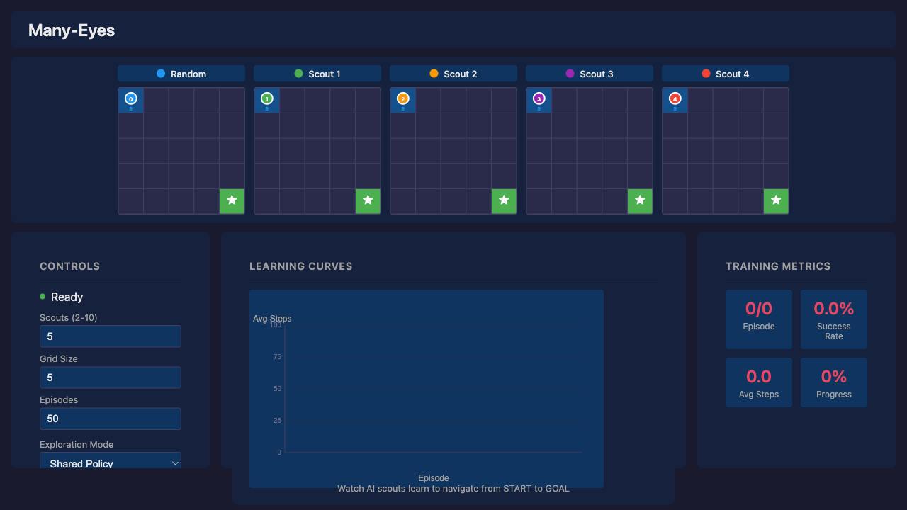
How It Works
The web version uses Q-learning with a shared Q-table (simpler than DQN for clarity). All scouts contribute to the same Q-table—the core “many eyes” concept: more explorers = faster Q-value convergence.
Scout Role Epsilon Behavior Random Baseline 1.0 (constant) Always random, never follows policy Scouts 1-N Learning Agents 0.5-0.8 → 0.01 Epsilon-greedy with decay Exploration Modes
The UI provides a dropdown to select different exploration strategies:
Mode Heatmap Diversity Learning Performance Shared Policy Low (identical paths) Best (lowest avg steps) Diverse Paths High (distinct paths) Worse (biases override optimal) High Exploration High Worst (never fully exploits) Boltzmann Moderate Moderate The Diversity vs Performance Trade-off
There’s a fundamental trade-off between visual diversity and learning performance:
-
Shared Policy wins on performance: The “many eyes” benefit comes from diverse exploration during learning (finding the goal faster). But once Q-values converge, all scouts should follow the same optimal policy.
-
Diverse Paths sacrifices performance for visuals: Scout-specific directional biases (Scout 1 prefers right, Scout 2 prefers down) create visually interesting heatmaps but suboptimal behavior.
-
High Exploration never converges: Fixed 50% random actions means scouts never fully exploit the learned policy.
Key insight: For best learning, use Shared Policy. Use other modes to visualize how different exploration strategies affect the learning process, but expect higher average steps.
Learning Phases
Phase Episodes Avg Steps Behavior Random 1-5 ~70 All scouts exploring randomly Early Learning 5-15 40-60 Policy starts forming Convergence 15-30 15-25 Clear optimal path emerges Stable 30+ 12-18 Near-optimal with random scout noise Why “Average Steps to Goal”?
Success rate is coarse-grained—with 5 scouts, only 6 values are possible (0%, 20%, 40%, 60%, 80%, 100%). After ~10 episodes, all scouts typically reach the goal. Average steps shows continued policy refinement, dropping from ~70 (random) to ~8 (optimal).
Running the Visualization
./scripts/serve.sh # Open http://localhost:3200- Yew/WASM frontend with FastAPI backend
- Speed control from 1x to 100x
- Replay mode to step through recorded training
What’s Next
Potential future directions:
Direction Why It Matters Larger environments Test scaling to 15x15, 25x25 grids Scout communication Real-time sharing vs passive pooling Adaptive intrinsic rewards Learn the reward function (closer to full IRPO) Multi-goal environments Multiple sparse rewards to discover Key Takeaways
-
Intrinsic rewards drive exploration. CuriousScout and OptimisticScout implement different philosophies: novelty bonuses vs optimistic initialization.
-
Strategy quality > diversity in simple environments. Five good scouts beat five diverse but weaker scouts.
-
Diversity during learning, convergence after. The “many eyes” benefit comes from diverse exploration during learning. Once Q-values converge, all scouts should follow the same optimal policy.
-
Shared Q-table enables collective learning. All scouts contribute to one Q-table—more explorers means faster convergence.
-
Visual diversity costs performance. Modes like “Diverse Paths” create interesting heatmaps but suboptimal behavior. Use “Shared Policy” for best learning results.
References
Concept Paper IRPO Intrinsic Reward Policy Optimization (Cho & Tran 2026) Reagent Reasoning Reward Models for Agents (Fan et al. 2026) ICM Curiosity-driven Exploration (Pathak et al. 2017)
Diverse exploration, convergent execution. Many eyes see more, but the best path is the one they all agree on.
Part 6 of the Machine Learning series. View all parts | Next: Part 7 →
Comments or questions? SW Lab Discord or YouTube @SoftwareWrighter.
-
597 words • 3 min read • Abstract
How AI Learns Part 1: The Many Meanings of Learning

When people say, “AI learned something,” they usually mean one of at least four very different things.
Large Language Models (LLMs) do not learn in one single way. They learn at different time scales, in different locations, and with very different consequences. To understand modern AI systems—especially agents—we need to separate these layers.
Resource Link Related ICL Revisited | RLM | Engram Comments Discord Four Time Scales of Learning

Learning happens at different layers with different persistence and speed. 1. Pretraining (Years)
This is the foundation.
The model trains on massive datasets using gradient descent. The result is a set of weights—billions of parameters—encoding statistical structure of language and knowledge.
This learning:
- Is slow and expensive
- Persists across restarts
- Cannot easily be reversed
- Is vulnerable to interference if modified later
Think of this as long-term biological memory.
2. Fine-Tuning (Days to Weeks)
Fine-tuning modifies the weights further, but with narrower data.
This includes:
- Instruction tuning (following directions)
- Alignment methods (Reinforcement Learning from Human Feedback (RLHF), Direct Preference Optimization (DPO))
- Domain adaptation
- Parameter-efficient methods like Low-Rank Adaptation (LoRA)
This is still weight-based learning.
It persists across restarts. It risks catastrophic forgetting. It modifies the brain itself.
3. Memory-Based Learning (Seconds to Minutes)
This is where many modern systems shift.
Instead of changing weights, they store information externally:
- RAG (Retrieval-Augmented Generation)
- CAG (Cache-Augmented Generation)
- Vector databases
- Engram-style memory modules
The model retrieves relevant memory per query.
The brain stays stable. The notebook grows.
This learning:
- Persists across restarts
- Survives model upgrades
- Does not cause forgetting
- Is fast
4. In-Context Learning (Milliseconds)
This is temporary reasoning scaffolding.
Information exists only in the prompt window.
It:
- Does not update weights
- Does not persist across sessions
- Is powerful but fragile
- Suffers from context rot
This is working memory.
Why This Matters
Most discussions collapse all of this into “the model learned.”
But:
- Updating weights risks forgetting
- Updating memory does not
- Updating prompts does not persist
- Updating adapters can be modular and reversible
Continuous learning systems must coordinate all four.
Persistence Comparison
Mechanism Persists Across Chat? Persists Across Restart? Persists Across Model Change? Pretraining Yes Yes No Fine-tune Yes Yes No LoRA Yes Yes Usually Distillation Yes Yes No ICL No No No RAG Yes Yes Yes Engram Yes Yes Yes CAG Yes Yes Yes That last column is subtle but powerful for agents.
References
Concept Paper LoRA LoRA: Low-Rank Adaptation of Large Language Models (Hu et al. 2021) RAG Retrieval-Augmented Generation for Knowledge-Intensive NLP Tasks (Lewis et al. 2020) ICL What Can Transformers Learn In-Context? (Garg et al. 2022) Engram Engram: Conditional Memory via Scalable Lookup (DeepSeek 2025) DPO Direct Preference Optimization (Rafailov et al. 2023) Coming Next
In Part 2, we’ll examine the two fundamental failure modes that arise from confusing these layers: catastrophic forgetting and context rot.
Learning happens in layers of permanence.
Part 1 of the How AI Learns series. View all parts | Next: Part 2 →
Comments or questions? SW Lab Discord or YouTube @SoftwareWrighter.
-
1155 words • 6 min read • Abstract
music-pipe-rs: Unix Pipelines for MIDI Composition

After building midi-cli-rs for quick mood-based generation, I wanted something more surgical. What if music generation worked like Unix commands—small tools connected by pipes?
Resource Link Code music-pipe-rs Related midi-cli-rs Next Web Demo and Multi-Instrument Comments Discord The Unix Philosophy for Music
Most generative music tools are monolithic. You get one application with a closed workflow. If you want to inspect intermediate results, you can’t. If you want to swap one transformation for another, you rebuild everything.
Unix solved this decades ago: small tools that do one thing well, connected by pipes. Each tool reads from stdin, writes to stdout. You can inspect any point in the pipeline with
head, filter withgrep, transform withjq.music-pipe-rs applies this philosophy to MIDI composition.
A Pipeline in Action
seed 12345 | motif --notes 16 --bpm 120 | humanize | to-midi --out melody.midFour stages:
- seed establishes the random seed for the entire pipeline
- motif generates a melodic pattern (using the pipeline seed)
- humanize adds timing and velocity variation (using the same seed)
- to-midi converts the event stream to a standard .mid file
The output plays in any DAW.
Seed-First Architecture
The
seedstage goes at the head of the pipeline:# Explicit seed for reproducibility seed 12345 | motif --notes 16 | humanize | to-midi --out melody.mid # Auto-generated seed (printed to stderr) seed | motif --notes 16 | humanize | to-midi --out melody.mid # stderr: seed: 1708732845All downstream stages read the seed from the event stream. No
--seedarguments scattered across the pipeline. One seed, set once, used everywhere.This means:
- Same seed = identical output across all random stages
- Different seed = different composition with same structure
- Reproducibility is trivial: just save the seed number
JSONL: The Intermediate Format
Between stages, events flow as JSONL (JSON Lines). Each line is a complete event:
{"type":"Seed","seed":12345}
{"type":"NoteOn","t":0,"ch":0,"key":60,"vel":80}
{"type":"NoteOff","t":480,"ch":0,"key":60}
This format is human-readable and tool-friendly:
# See the first 10 events
seed 42 | motif --notes 8 | head -10

# Count how many NoteOn events
seed 42 | motif --notes 16 | grep NoteOn | wc -l

# Pretty-print with jq
seed 42 | motif --notes 4 | jq .
No binary formats to decode. No proprietary protocols. Just text.
Visualization with viz
The
vizstage prints a sparkline to stderr while passing events through:seed 12345 | motif --notes 16 | viz | humanize | to-midi --out melody.midOutput on stderr:
▃▅▇▅▃▁▂▄▆▇▆▄▂▁▃▅For more detail, use piano roll mode:
seed 12345 | motif --notes 16 | viz --rollG6 │···█············│ F#6 │·····█··········│ F6 │····█···········│ G5 │·██·········█···│ F5 │···········█····│ E5 │·········██···█·│ C5 │█·····███····█·█│The visualization goes to stderr; the JSONL events continue to stdout. You can inspect the music without breaking the pipeline.
Available Stages
Stage Type Description seedStart Establish random seed for pipeline motifGenerate Create melodic patterns euclidGenerate Euclidean rhythm generation transposeTransform Shift notes by semitones scaleTransform Constrain notes to a scale humanizeTransform Add timing/velocity variation vizInspect Print sparkline visualization to-midiOutput Convert to .mid file Each stage is a separate binary. Mix and match as needed.
Euclidean Rhythms
The
euclidstage generates Euclidean rhythms—mathematically optimal distributions of hits across steps:# 3 hits distributed across 8 steps (Cuban tresillo) seed | euclid --pulses 3 --steps 8 --note 36 | to-midi --out kick.mid # 4-on-the-floor kick pattern seed | euclid --pulses 4 --steps 16 --note 36 | to-midi --out four-floor.midThese patterns appear in music worldwide because they “feel right”—the spacing is as even as possible.
Scale Locking
The
scalestage constrains notes to a musical scale:seed 42 | motif --notes 16 | scale --root C --mode minor | to-midi --out c-minor.midNo wrong notes. Every pitch fits the harmonic context.
Layering Streams
Generate drum and melody separately, then combine:
{
    seed 100 | euclid --pulses 4 --steps 16 --note 36 --ch 9;
    seed 100 | motif --notes 16 | scale --root C --mode pentatonic;
} | to-midi --out layered.mid
Channel 9 is General MIDI drums. Same seed ensures coherence between parts. Both streams merge into a single MIDI file.
Why Not Just Use midi-cli-rs?
Different tools for different needs:
Tool Strength Use Case midi-cli-rs Quick mood presets “Give me 5 seconds of jazz” music-pipe-rs Compositional control “Generate a motif, constrain to scale, add swing” midi-cli-rs is high-level: pick a mood, get music. music-pipe-rs is low-level: build compositions from primitive operations.
Both are useful. Both work with AI coding agents.
The Personal Software Pattern
This continues the theme: build small tools that compose well. Don’t try to solve everything in one application. Let Unix handle orchestration.
The best part? Standard tools still work.
head,grep,jq,wc—all participate in the pipeline. No special music knowledge required to inspect the data.
Disclaimer
You are responsible for how you use generated audio. Ensure you have the appropriate rights and permissions for any commercial or public use. This tool generates MIDI data algorithmically—how you render and distribute the final audio is your responsibility.
Be aware that algorithmic composition can inadvertently produce sequences similar to existing copyrighted works. Whether you use this tool, AI generation, or compose by hand, you must verify that your output doesn’t infringe on existing copyrights before public release or commercial use. Protect yourself legally.
Part 4 of the Personal Software series. View all parts | Next: Part 5 →
Comments or questions? SW Lab Discord or YouTube @SoftwareWrighter.
-
452 words • 3 min read • Abstract
Five ML Concepts - #21

5 machine learning concepts. Under 30 seconds each.
Resource Link Papers Links in References section Video Five ML Concepts #21 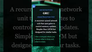
Comments Discord References
Concept Reference Prompt Injection Prompt Injection attack against LLM-integrated Applications (Liu et al. 2023) Jailbreaks Jailbroken: How Does LLM Safety Training Fail? (Wei et al. 2023) GRU Empirical Evaluation of Gated Recurrent Neural Networks (Chung et al. 2014) Planning vs Prediction Between accurate prediction and poor decision making (Zaffalon et al. 2023) Production Rollbacks MLOps best practice (no canonical paper) Today’s Five
1. Prompt Injection
Malicious instructions embedded in user input that override intended system behavior. An attacker crafts text that tricks an AI into ignoring its original instructions.
This is a major security concern for LLM-integrated applications.
Like slipping a forged instruction into a trusted document.
2. Jailbreaks
Techniques that attempt to bypass safety constraints in AI systems. These attacks exploit gaps between a model’s capabilities and its safety training.
Safety training can fail due to competing objectives or mismatched generalization.
Like convincing a guard to bend the rules.
3. GRU (Gated Recurrent Unit)
A recurrent neural network unit with gates that control memory flow. GRUs decide what information to keep and what to discard at each time step.
Simpler than LSTM but designed for similar sequence modeling tasks.
Like a notepad where you decide what to keep and what to erase.
4. Planning vs Prediction
Prediction forecasts likely outcomes. Planning evaluates actions across possible futures. Accurate predictions don’t guarantee good decisions—you also need to model how actions affect outcomes.
This is a key gap in many AI/ML systems.
Like knowing it will rain versus deciding whether to bring an umbrella.
5. Production Rollbacks
Reverting to a previous stable model version after deployment issues. When a new model causes problems in production, rolling back quickly minimizes impact.
Essential MLOps practice for maintaining system reliability.
Like reloading a saved game state when something breaks.
Quick Reference
Concept One-liner Prompt Injection Malicious instructions overriding AI behavior Jailbreaks Bypassing safety constraints GRU Gated memory for sequence modeling Planning vs Prediction Action evaluation vs forecasting Production Rollbacks Reverting to stable model versions
Short, accurate ML explainers. Follow for more.
Part 21 of the Five ML Concepts series. View all parts | Next: Part 22 →
Comments or questions? SW Lab Discord or YouTube @SoftwareWrighter.
-
1337 words • 7 min read • Abstract
midi-cli-rs: Extending with Custom Mood Packs

Personal Software doesn’t stop at “it works.” It evolves. After building midi-cli-rs for AI agents to generate music, I wanted more moods—without recompiling Rust every time.
The solution: a plugin system that lets anyone create custom mood packs using simple TOML files.
Resource Link Examples Listen to Samples Wiki Plugin Documentation Video Plugin Moods Explainer 
Code midi-cli-rs Comments Discord The Problem with Built-in Only
The original midi-cli-rs shipped with a handful of mood presets: suspense, eerie, upbeat, calm, ambient, jazz. Useful, but limited. What if you want synthwave? Chillout? Something faster or in a different key?
Hardcoding every possible mood isn’t practical. And asking users to modify Rust source code isn’t friendly.
Three Levels of Extensibility
Level What You Get What You Change Skill Required ✓ Built-in Moods 9 curated generators Nothing—use as-is None ✓ Plugin Moods Parameter variations TOML config files Text editing ✗ Custom Generators New musical patterns Rust source code Programming (future) This post covers Plugin Moods—the middle tier. You can preset combinations of tempo, key, and intensity, but you’re still using the built-in generators’ musical logic. Want a “smooth-jazz” preset (slower, mellower)? Plugin mood. Want bebop or Latin jazz with different chord progressions? That requires a custom generator.
Custom generators (writing new Rust code) will be covered in a future post when the plugin editor ships.
The Plugin Architecture
Custom moods live in
~/.midi-cli-rs/moods/as TOML files. Each file is a “mood pack” that can define multiple moods. The CLI discovers them automatically.Here’s how it works:
~/.midi-cli-rs/
└── moods/
    ├── electronic.toml    # Your synthwave, techno, etc.
    ├── cinematic.toml     # Epic, tension, wonder
    └── seasonal.toml      # Holiday themes
Creating a Mood Pack
A plug-in mood pack has two parts: pack metadata and mood definitions.
[pack]
name = "electronic"
version = "1.0.0"
author = "Your Name"
description = "Electronic music styles"

[[moods]]
name = "synthwave"
base_mood = "upbeat"
default_tempo = 118
default_key = "Am"
default_intensity = 65
description = "80s synthwave vibes"
tags = ["electronic", "retro"]

[[moods]]
name = "chillout"
base_mood = "ambient"
default_tempo = 85
default_key = "Em"
default_intensity = 40
description = "Relaxed electronic"
Each mood delegates to a built-in generator (
base_mood) but overrides specific parameters. You get the musical logic of the built-in mood with your customizations applied.Available Base Moods
Your custom moods can extend any of the nine built-in generators:
Base Mood Character suspenseTense, building eerieDark, unsettling upbeatEnergetic, positive calmPeaceful, slow ambientAtmospheric, textural jazzSwing, improvisation chiptune8-bit, retro gaming orchestralClassical instruments showBroadway, theatrical Configuration Options
Each mood definition supports these overrides:
Field Description Example nameCLI name (required) "synthwave"base_moodBuilt-in to extend (required) "upbeat"default_tempoBPM 118default_keyMusical key "Am","C","Eb"default_intensity0-100 energy level 65descriptionHuman-readable description "80s vibes"tagsDiscovery tags ["electronic", "retro"]How Seeds Create Variation
Seeds aren’t random—they’re deterministic variation selectors. The same mood + same seed always produces identical output. But different seeds create observable musical differences across multiple dimensions:
Parameter Variation Range Tempo ±15% from base Layer inclusion Which instruments appear Melodic contour 16 different phrase shapes Note density 0.6x to 1.4x Rest probability 0% to 35% silence Phrase length 3-8 notes Velocity -15 to +15 offset The system uses hash-based mixing with unique salts for each parameter. This means adjacent seeds (42 vs 43) produce completely different outputs—no gradual transitions between seeds.
When you combine plugin moods with seed variation, you get a matrix: your custom tempo/key/intensity settings applied across different seed-driven variations of the underlying generator’s patterns.
Using Custom Moods
Once your TOML file is in place, the mood appears automatically:
# List all moods (built-in + plugins)
midi-cli-rs moods

# Generate with your custom mood
midi-cli-rs preset -m synthwave -d 5 -s 42 -o output.wav
The seed system still works—same mood + same seed = identical output.
Example: Electronic Pack
Here’s a complete pack with four electronic moods:
[pack]
name = "electronic"
version = "1.0.0"
description = "Electronic music styles"

[[moods]]
name = "synthwave"
base_mood = "upbeat"
default_tempo = 118
default_key = "Am"
default_intensity = 65

[[moods]]
name = "chillout"
base_mood = "ambient"
default_tempo = 85
default_key = "Em"
default_intensity = 40

[[moods]]
name = "techno"
base_mood = "upbeat"
default_tempo = 130
default_key = "Dm"
default_intensity = 85

[[moods]]
name = "8bit"
base_mood = "chiptune"
default_tempo = 140
default_key = "C"
default_intensity = 70
Drop this in
~/.midi-cli-rs/moods/electronic.tomland you have four new moods.What’s Next
This plugin system handles mood variations—different tempos, keys, and intensities applied to existing generators. A future update will add a plugin editor for creating entirely new musical patterns without writing Rust.
For now, the delegation model covers most use cases: want faster jazz? Darker ambient? Major-key suspense? Create a TOML file and you’re done.
The Personal Software Pattern
This follows the Personal Software philosophy: start with something that works, then extend it as needs emerge. The plugin system wasn’t in the original design. It grew from actual use—wanting more moods without recompiling.
Good personal software leaves room to grow.
Disclaimer
You are responsible for how you use generated audio. Ensure you have the appropriate rights and permissions for any commercial or public use. This tool generates MIDI data algorithmically—how you render and distribute the final audio is your responsibility.
Be aware that algorithmic composition can inadvertently produce sequences similar to existing copyrighted works. Whether you use this tool, AI generation, or compose by hand, you must verify that your output doesn’t infringe on existing copyrights before public release or commercial use. Protect yourself legally.
Part 3 of the Personal Software series. View all parts | Next: Part 4 →
Comments or questions? SW Lab Discord or YouTube @SoftwareWrighter.
-
461 words • 3 min read • Abstract
Five ML Concepts - #20

5 machine learning concepts. Under 30 seconds each.
Resource Link Papers Links in References section Video Five ML Concepts #20 
Comments Discord References
Concept Reference VAEs Auto-Encoding Variational Bayes (Kingma & Welling 2013) Uncertainty Estimation What Uncertainties Do We Need in Bayesian Deep Learning? (Kendall & Gal 2017) Interpretability Towards A Rigorous Science of Interpretable Machine Learning (Doshi-Velez & Kim 2017) Gradient Noise Stochastic Gradient Descent as Approximate Bayesian Inference (Mandt et al. 2017) Human-in-the-Loop Human-in-the-Loop Machine Learning (Monarch 2021) Today’s Five
1. Variational Autoencoders (VAEs)
VAEs are probabilistic autoencoders that learn a structured latent distribution. By sampling from that distribution, they can generate new examples similar to the training data.
The key innovation is regularizing the latent space to be smooth and continuous.
Like learning not just to summarize books, but to create new ones in a similar style.
2. Uncertainty Estimation
Models can estimate how confident they should be in predictions. Some uncertainty comes from noisy data (aleatoric), and some from limited knowledge (epistemic).
Knowing when a model is uncertain enables safer decision-making.
Like a weather forecast giving seventy percent chance of rain instead of a simple yes or no.
3. Why Interpretability Is Hard
Neural networks represent information across many interacting parameters. No single component cleanly maps to a human concept.
Distributed representations enable powerful learning but resist simple explanations.
Like trying to explain a dream by pointing to individual neurons.
4. Gradient Noise
When training with mini-batches, gradients vary from step to step. A little noise can help exploration, but too much can slow convergence.
Batch size, learning rate, and gradient clipping all influence this noise level.
Like getting slightly different directions each time you ask for help.
5. Human-in-the-Loop Systems
Humans review, supervise, or override model decisions in critical workflows. This improves safety and accountability in high-stakes applications.
The approach combines model efficiency with human judgment where it matters most.
Like a pilot monitoring autopilot and stepping in when necessary.
Quick Reference
Concept One-liner VAEs Generative models with structured latent spaces Uncertainty Estimation Know when you don’t know Interpretability Distributed representations resist explanation Gradient Noise Mini-batch variation in training Human-in-the-Loop Human oversight for critical decisions
Short, accurate ML explainers. Follow for more.
Part 20 of the Five ML Concepts series. View all parts | Next: Part 21 →
Comments or questions? SW Lab Discord or YouTube @SoftwareWrighter.
-
648 words • 4 min read • Abstract
In-Context Learning Revisited: From Mystery to Engineering
It was 2020 when GPT-3 shocked everyone. It could learn from examples in the query—without updating its weights. We called it In-Context Learning. But was it magic, or was it doing something deeper?
Resource Link Video ICL Revisited 
Papers 4 References Comments Discord Phase 1: The Empirical Discovery (2020)
The GPT-3 paper showed that large models could perform few-shot learning. Give them examples, and they generalize. No gradient updates. No retraining. Just forward passes.
The surprising part was that scaling alone seemed to unlock it.
Paper: Language Models are Few-Shot Learners
ELI5: Show a big language model a few examples of a task in your prompt, and it figures out how to do the task—without any retraining. Nobody told it to do this. It just emerged when models got big enough.
Main idea: Scale unlocks emergent capabilities. ICL was discovered, not designed.
Phase 2: Mechanistic Explanations (2022)
By 2022, researchers began probing the internal mechanisms. Several papers proposed that transformers implement implicit meta-learning. The model appears to learn during inference by performing gradient-descent-like operations internally.
Paper: What Explains In-Context Learning in Transformers?
ELI5: When you give a transformer examples, its attention layers do something that looks like fitting a simple linear model to those examples—on the fly, during the forward pass. It’s not memorizing; it’s computing a mini-solution.
Main idea: ICL works because attention can simulate linear regression internally.
Paper: Transformers Learn In-Context by Gradient Descent
ELI5: The transformer’s forward pass is secretly doing something similar to training. The attention mechanism acts like one step of gradient descent over the examples you provided. Learning happens inside inference.
Main idea: ICL is implicit gradient descent—learning hidden inside prediction.
Phase 3: Engineering the Effect
Once researchers understood that ordering and structure affect ICL, prompt design became less of an art and more of an optimization problem. The quality and arrangement of demonstrations directly shape performance.
ICL became tunable. Researchers could now deliberately improve it rather than just observe it.
Phase 4: Interactive ICL (2026)
Recent work pushes this further. Models are trained to predict natural language critiques and feedback. If a model can predict what a teacher would say, it can internalize that signal. External correction becomes an internal capability.
Paper: Improving Interactive In-Context Learning from Natural Language Feedback
ELI5: Train a model to guess what feedback a human would give. Now the model has internalized the “teacher” and can improve itself without needing the actual teacher present. Self-correction without weight updates.
Main idea: Models can learn to learn from feedback, making ICL interactive and self-improving.
Beyond Language
Newer work applies ICL to neuroscience discovery, showing that the mechanism is not limited to text tasks. It becomes a flexible reasoning substrate across domains. That’s when you know a concept has matured.
The Arc
Phase Era Key Insight Discovery 2020 Emerges from scale Explanation 2022 Implicit gradient descent Engineering 2023-24 Prompt design as optimization Self-improvement 2026 Learning from feedback The Deeper Insight
In-Context Learning started as an emergent surprise. Now it’s becoming an engineered learning substrate inside transformers.
It was not magic. It was meta-learning hiding in plain sight.
References
Paper Link Language Models are Few-Shot Learners (GPT-3) arXiv:2005.14165 What Explains In-Context Learning in Transformers? arXiv:2202.12837 Transformers Learn In-Context by Gradient Descent arXiv:2212.07677 Improving Interactive ICL from Natural Language Feedback arXiv:2602.16066
ICL started as “whoa, it works.” Now we understand “why it works.” Next: engineering it deliberately.
Part 5 of the Machine Learning series. View all parts | Next: Part 6 →
Comments or questions? SW Lab Discord or YouTube @SoftwareWrighter.
-
456 words • 3 min read • Abstract
Five ML Concepts - #19

5 machine learning concepts. Under 30 seconds each.
Resource Link Papers Links in References section Video Five ML Concepts #19 
Comments Discord References
Concept Reference Autoencoders Reducing the Dimensionality of Data with Neural Networks (Hinton & Salakhutdinov 2006) Correlation vs Causation Causality (Pearl 2009) Curriculum Learning Curriculum Learning (Bengio et al. 2009) Failure Analysis Practical Machine Learning for Computer Vision (Lakshmanan et al. 2021) Covariate Shift Dataset Shift in Machine Learning (Quinonero-Candela et al. 2009) Today’s Five
1. Autoencoders
Autoencoders are neural networks trained to compress inputs into a smaller representation and reconstruct them. The bottleneck forces the model to capture essential structure.
This learned compression is useful for dimensionality reduction, denoising, and feature learning.
Like summarizing a book into key points and then rebuilding the story from that summary.
2. Correlation vs Causation
Two variables can move together without one causing the other. Models typically learn correlations present in data, not true cause-and-effect relationships.
This matters because interventions based on correlation alone may not produce intended effects.
Like noticing umbrella sales rise with rain—umbrellas don’t cause rain.
3. Curriculum Learning
Training starts with easier examples and gradually introduces harder ones. This can improve stability and learning speed in some settings.
The approach mirrors how humans learn complex subjects incrementally.
Like teaching math by starting with addition before moving to calculus.
4. Failure Analysis
Failure analysis groups model errors into categories to understand where performance breaks down. This helps target improvements instead of guessing.
Systematic error analysis often reveals actionable patterns invisible in aggregate metrics.
Like a teacher reviewing which types of questions students miss most often.
5. Covariate Shift
Covariate shift occurs when the input distribution changes between training and deployment, while the task itself remains the same. The model may underperform because it sees unfamiliar inputs.
Monitoring input distributions helps detect this shift early.
Like training a driver in sunny weather and testing them in snow.
Quick Reference
Concept One-liner Autoencoders Compress and reconstruct to learn structure Correlation vs Causation Co-occurrence isn’t cause Curriculum Learning Start easy, progress to hard Failure Analysis Categorize errors to guide fixes Covariate Shift New inputs, same task
Short, accurate ML explainers. Follow for more.
Part 19 of the Five ML Concepts series. View all parts | Next: Part 20 →
Comments or questions? SW Lab Discord or YouTube @SoftwareWrighter.
-
2244 words • 12 min read • Abstract
JSON et al: A Deep Dive into Data Serialization Formats

JSON is everywhere. APIs. Logs. Databases. Configuration files. But it’s not alone. A whole ecosystem of formats exists—each optimizing for different tradeoffs.
This post expands on the JSON et al short, providing technical depth on each format: when it was created, where it’s specified, and what problems it solves.
The Tradeoff Triangle
Before diving in, understand the fundamental constraint. Data formats balance three competing goals:
Goal Description Human Readability Can a developer read and edit it directly? Compactness How many bytes does it take to represent data? Query Performance How fast can you access specific fields? You usually only get two. JSON optimizes readability. Protobuf optimizes compactness. JSONB optimizes query performance. No format wins everywhere.
JSON: The Ubiquitous Baseline
Created: 2001 (discovered/formalized by Douglas Crockford) Specification: ECMA-404 (2013), RFC 8259 (2017) File Extension:
.jsonJSON (JavaScript Object Notation) emerged from JavaScript’s object literal syntax but became language-agnostic. Crockford didn’t invent it—he “discovered” it already existing in JavaScript and formalized the specification.
Technical Details
- Encoding: UTF-8 text (UTF-16/32 allowed but rare)
- Data Types: Objects
{}, arrays[], strings, numbers, booleans,null - Schema: None required
- Comments: Not allowed in strict JSON
Strengths
- Universal parser support (every language has one)
- Human readable without tools
- Web-native (JavaScript parses it natively)
- Simple specification (fits on a business card)
Weaknesses
- Verbose (field names repeated for every object)
- No binary data type (must base64-encode)
- No comments (frustrating for config files)
- Parsing overhead (tokenization + string decoding every time)
ELI5
Like typing a long email instead of sending a terse text. Every message spells everything out—clear, but verbose.
When to Use
REST APIs, configuration (when comments aren’t needed), data interchange between systems, anywhere human readability matters more than efficiency.
JSONL / NDJSON: Streaming JSON
Created: ~2013 (formalized) Specification: JSON Lines, NDJSON File Extension:
.jsonl,.ndjsonJSONL (JSON Lines) and NDJSON (Newline-Delimited JSON) are the same concept: one valid JSON object per line, separated by newlines.
Technical Details
{"name": "Alice", "score": 95}
{"name": "Bob", "score": 87}
{"name": "Carol", "score": 92}
No wrapping array. Each line is independently parseable.
Strengths
- Streaming: Process line-by-line without loading entire file
- Append-only: Add records without rewriting the file
- Parallel processing: Split by line, distribute to workers
- Fault-tolerant: One corrupt line doesn’t invalidate the file
Weaknesses
- Not valid JSON (can’t parse with standard JSON parser)
- Still text-based (same verbosity as JSON)
- No random access by index
ELI5
Like removing one comma per line to save some typing. Each line is self-contained, so you can grab and process them one at a time.
When to Use
Log files, big data pipelines (Spark, Pandas), ML datasets, event streams, anywhere you need to process records incrementally.
JSONB: Binary JSON for Databases
Created: 2014 (PostgreSQL 9.4) Specification: Implementation-specific (no universal standard) Storage: Database column type
JSONB isn’t a file format—it’s a database storage optimization. PostgreSQL’s JSONB differs from MongoDB’s BSON, which differs from other implementations.
PostgreSQL JSONB Details
- Parsed once: Text converted to binary on INSERT
- Keys sorted: Deterministic ordering for indexing
- Duplicates removed: Last value wins
- Offset table: O(log n) field lookup instead of O(n) text scanning
MongoDB BSON
Specification: bsonspec.org
BSON (Binary JSON) is MongoDB’s serialization format. Unlike PostgreSQL’s JSONB, BSON is a standalone binary format:
- Type-prefixed values
- Supports additional types (Date, Binary, ObjectId)
- Length-prefixed for fast skipping
- ~10-15% smaller than JSON typically
Strengths
- Fast queries without re-parsing
- Indexable (GIN indexes on JSONB in PostgreSQL)
- Type coercion at storage time
Weaknesses
- Not portable (implementation-specific)
- Not human-readable
- INSERT overhead (parsing cost upfront)
ELI5
Instead of cooking from scratch every time, you heat a pre-made meal. The prep work happens once (on INSERT), so serving (queries) is fast.
When to Use
Database storage where you query into JSON structures. PostgreSQL JSONB + GIN indexes enable fast
@>containment queries.
Protocol Buffers: Google’s Schema-First Format
Created: 2001 (internal Google), 2008 (open-sourced) Specification: developers.google.com/protocol-buffers File Extension:
.proto(schema), binary wire formatProtocol Buffers (Protobuf) is Google’s language-neutral, schema-required serialization format. It powers gRPC.
Technical Details
Schema definition:
message Sensor {
  int32 temperature = 1;
  int32 humidity = 2;
}
Wire format uses field numbers, not names:
Field 1: 72
Field 2: 40
Key Features
- Varint encoding: Small integers use fewer bytes
- Field numbers: Enable backward compatibility
- Code generation:
.proto→ language-specific classes - No self-description: Receiver must know schema
Strengths
- Extremely compact (3-10x smaller than JSON typically)
- Fast serialization/deserialization
- Strong versioning semantics
- gRPC integration
Weaknesses
- Requires schema agreement
- Not human-readable
- Tooling required for debugging
- Schema evolution has rules
ELI5
Everyone agrees upfront what “field 1” means. You don’t waste space spelling out “temperature”—you just send the number 1 and the value. Both sides know the code.
When to Use
Microservices (gRPC), internal APIs, anywhere bandwidth and latency matter more than debuggability.
ASN.1: The Telecom Veteran
Created: 1984 (ITU-T X.208) Specification: ITU-T X.680-X.683 Encoding Rules: BER, DER, PER, XER, and more
ASN.1 (Abstract Syntax Notation One) predates all modern formats. It defines both schema and encoding, with multiple encoding rules for different use cases.
Encoding Rules Comparison
Rule Use Case BER (Basic Encoding Rules) Flexible, general purpose DER (Distinguished Encoding Rules) Deterministic, for cryptography PER (Packed Encoding Rules) Most compact, for bandwidth-constrained XER (XML Encoding Rules) XML-based, for interop Where You See ASN.1
- X.509 certificates (SSL/TLS certs are DER-encoded ASN.1)
- LDAP (directory services)
- SNMP (network management)
- Telecom protocols (SS7, GSM, LTE)
Strengths
- Bit-level precision
- Proven over 40 years
- Multiple encoding options
- Formal verification possible
Weaknesses
- Complex specification
- Steep learning curve
- Tooling can be expensive
- Security vulnerabilities in parsers (historically)
ELI5
Same idea as Protobuf—everyone agrees upfront what each field number means. ASN.1 just got there 20 years earlier and handles even more edge cases.
When to Use
You probably won’t choose ASN.1 for new projects. You’ll encounter it in cryptography, certificates, and legacy telecom systems.
YAML: Human-Friendly Configuration
Created: 2001 (Clark Evans, Ingy döt Net, Oren Ben-Kiki) Specification: yaml.org/spec/1.2.2 File Extension:
.yaml,.ymlYAML (YAML Ain’t Markup Language) prioritizes human readability. It’s a superset of JSON—any valid JSON is valid YAML.
Technical Details
# Comments allowed!
server:
  host: localhost
  port: 8080
  features:
    - auth
    - logging
Key Features
- Indentation-based: Whitespace matters
- Comments:
#for single-line - Anchors/aliases:
&nameand*namefor references - Multiple documents:
---separator
Strengths
- Highly readable
- Comments supported
- Multi-line strings without escaping
- Complex data structures
Weaknesses
- “Norway problem”:
NOparses as booleanfalse - Whitespace sensitivity causes errors
- Multiple ways to express same data
- Security concerns (arbitrary code execution in some parsers)
ELI5
Optimized for clarity, not bandwidth. YAML is for humans editing config files—not for machines exchanging data over networks.
When to Use
Configuration files (Kubernetes, Docker Compose, CI/CD), anywhere humans edit data directly and comments help.
TOML: Minimal Configuration
Created: 2013 (Tom Preston-Werner) Specification: toml.io File Extension:
.tomlTOML (Tom’s Obvious Minimal Language) emerged as a reaction to YAML’s complexity. It’s used by Rust (Cargo.toml), Python (pyproject.toml), and others.
Technical Details
[server]
host = "localhost"
port = 8080

[server.features]
auth = true
logging = true
Key Features
- Explicit typing: Dates, times, arrays have clear syntax
- Sections:
[section]and[section.subsection] - No anchors: Intentionally simpler than YAML
- Deterministic: Same data = same representation
Strengths
- Easy to read and write
- Unambiguous parsing
- Clear error messages
- Growing ecosystem support
Weaknesses
- Less expressive than YAML
- Nested structures can be verbose
- Smaller ecosystem than JSON/YAML
ELI5
Same goal as YAML—clarity for humans, not bandwidth for machines—but with stricter rules so you make fewer mistakes.
When to Use
Configuration files where YAML’s complexity isn’t needed. Rust projects (mandatory). Python packaging (pyproject.toml).
TOON: Token-Optimized for LLMs
Created: October 2025 (toon-format organization) Specification: github.com/toon-format/toon (v3.0) File Extension:
.toonMedia Type:text/toon(provisional)TOON (Token Oriented Object Notation) is the newest format in this list, designed specifically for LLM input. It’s a lossless representation of JSON that minimizes tokens.
Technical Details
TOON combines YAML-style indentation for nested objects with CSV-like tabular layouts for uniform arrays:
users[2]{name,age}:
Alice,25
Bob,30
Equivalent JSON:
{"users": [{"name": "Alice", "age": 25}, {"name": "Bob", "age": 30}]}Key Features
- Header-based: Field names declared once, values follow
- 40% fewer tokens: Than equivalent JSON typically
- Lossless: Round-trips to JSON perfectly
- UTF-8 always: No encoding ambiguity
Performance
Metric JSON TOON Accuracy 69.7% 73.9% Efficiency (acc/1K tokens) 15.3 26.9 Strengths
- Significant token savings at scale
- Better context window utilization
- Lower API costs for LLM applications
- Human-readable (unlike binary formats)
Weaknesses
- New format (October 2025)
- Limited tooling compared to JSON
- Requires conversion layer for existing systems
- Not yet widely adopted
ELI5
Like having one header row for each column in a table instead of repeating the column name for every single row. You declare field names once, then just list the values.
When to Use
LLM prompts with structured data, RAG applications, anywhere token efficiency matters. Especially useful for large datasets with uniform object arrays.
Implementations
- TypeScript: Reference implementation
- Python: toons (Rust-based, fast)
- Go, Rust, .NET: Available via toon-format org
Alternatives Not in the Video
MessagePack
Created: 2008 (Sadayuki Furuhashi) Specification: msgpack.org
Binary JSON without schema. Type-prefixed values, efficient numeric encoding.
Use when: You want JSON semantics but smaller/faster.
CBOR
Created: 2013 (IETF) Specification: RFC 8949
Concise Binary Object Representation. Designed for constrained environments (IoT).
Use when: Resource-constrained devices, need a standard binary format.
Apache Avro
Created: 2009 (Apache, Doug Cutting) Specification: avro.apache.org
Schema-based, row-oriented binary format. Schema embedded or stored separately. Strong schema evolution support.
Use when: Big data pipelines (Hadoop, Kafka), schema evolution is critical.
Apache Parquet
Created: 2013 (Twitter + Cloudera) Specification: parquet.apache.org
Columnar storage format. Not for serialization—for analytics storage.
Use when: Large-scale analytics, data warehousing, Spark/Pandas workflows.
Cap’n Proto
Created: 2013 (Kenton Varda, ex-Protobuf author) Specification: capnproto.org
Zero-copy serialization. The serialized form is the in-memory form.
Use when: Extreme performance requirements, inter-process communication.
FlatBuffers
Created: 2014 (Google) Specification: google.github.io/flatbuffers
Zero-copy like Cap’n Proto but with better tooling. Used in games, mobile.
Use when: Games, mobile apps, anywhere memory allocation matters.
Quick Reference
Format Year Schema Binary Human-Readable Best For JSON 2001 No No Yes APIs, interchange JSONL 2013 No No Yes Logs, streaming JSONB 2014 No Yes No Database queries Protobuf 2008 Yes Yes No Microservices ASN.1 1984 Yes Yes No Crypto, telecom YAML 2001 No No Yes Config files TOML 2013 No No Yes Simple config TOON 2025 No No Yes LLM prompts MessagePack 2008 No Yes No Fast JSON CBOR 2013 Optional Yes No IoT Avro 2009 Yes Yes No Big data
Key Takeaways
-
No “best” format exists. Each optimizes for different constraints.
-
Text formats favor humans. JSON, YAML, TOML prioritize readability over efficiency.
-
Binary formats favor machines. Protobuf, MessagePack, CBOR prioritize compactness and speed.
-
Schema formats favor correctness. Protobuf, Avro, ASN.1 catch errors at compile time.
-
The tradeoff triangle is real. Readability, compactness, query performance—pick two.
The question isn’t “which format wins?” The question is: what problem are you solving?
Resources
- ECMA-404 JSON Specification
- RFC 8259 JSON
- JSON Lines Specification
- PostgreSQL JSONB Documentation
- Protocol Buffers Documentation
- YAML 1.2.2 Specification
- TOML v1.0.0 Specification
- RFC 8949 CBOR
- MessagePack Specification
- Apache Avro Specification
Data formats are design decisions. Choose based on your constraints, not trends.
Part 2 of the General Technology series. View all parts | Next: Part 3 →
Comments or questions? SW Lab Discord or YouTube @SoftwareWrighter.
-
449 words • 3 min read • Abstract
Five ML Concepts - #18

5 machine learning concepts. Under 30 seconds each.
Resource Link Papers Links in References section Video Five ML Concepts #18 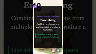
Comments Discord References
Concept Reference Preference Learning Learning to summarize from human feedback (Stiennon et al. 2020) Ensembling Ensemble Methods in Machine Learning (Dietterich 2000) ML Fragility Distribution Shift (Quinonero-Candela et al. 2009) Epoch Deep Learning (Goodfellow et al. 2016), Chapter 8 Cost vs Quality Efficient Transformers: A Survey (Tay et al. 2022) Today’s Five
1. Preference Learning
Instead of learning from fixed labels, models are trained from comparisons between outputs. This helps align model behavior with human judgments.
The approach works well when absolute quality is hard to define but relative preferences are easier to express.
Like learning to cook by asking which dish tastes better.
2. Ensembling
Ensembling combines predictions from multiple models. Different models make different errors, and combining them can improve robustness.
Common strategies include voting, averaging, and stacking models together.
Like asking several experts and averaging their opinions.
3. Why ML Is Fragile
Models rely on statistical patterns learned from data. When those patterns shift, performance can degrade quickly.
This fragility emerges because models optimize for training distributions, not arbitrary future scenarios.
Like a spell checker that works on common words but struggles with unusual ones.
4. Epoch
An epoch is one complete pass through the training dataset. Multiple epochs allow the model to refine its weights over repeated passes.
Training typically continues for many epochs until validation performance stops improving.
Like reading a textbook from beginning to end more than once.
5. Cost vs Quality Tradeoffs
Increasing model size or compute often improves performance, but also increases cost and latency. Engineers balance quality against budget and responsiveness.
Production systems often use smaller, faster models rather than the largest available.
Like choosing between a luxury car and an economy car depending on your needs.
Quick Reference
Concept One-liner Preference Learning Train from comparisons, not labels Ensembling Combine models for robustness ML Fragility Statistical models break on distribution shift Epoch One pass through training data Cost vs Quality Bigger isn’t always better in production
Short, accurate ML explainers. Follow for more.
Part 18 of the Five ML Concepts series. View all parts | Next: Part 19 →
Comments or questions? SW Lab Discord or YouTube @SoftwareWrighter.
-
1043 words • 6 min read • Abstract
midi-cli-rs: Music Generation for AI Coding Agents

AI coding agents can write code, generate images, and produce text. But what about music? When I needed background audio for explainer videos, I wanted a tool that AI agents could use directly—no music theory required.
Resource Link Video midi-cli-rs Explainer 
Examples Listen to Samples Code midi-cli-rs Comments Discord The Problem
Generating music programmatically is hard. Traditional approaches require understanding music theory, MIDI specifications, instrument mappings, and audio synthesis. That’s a lot to ask of an AI agent that just needs a 5-second intro.
I wanted something simpler: a CLI tool where an agent could say “give me 5 seconds of suspenseful music” and get a usable WAV file.
The Solution: Mood Presets
midi-cli-rs solves this with mood presets—curated musical generators that produce complete compositions from a single command:
# Generate a 5-second suspenseful intro
midi-cli-rs preset --mood suspense --duration 5 -o intro.wav

# Upbeat outro with specific key
midi-cli-rs preset -m upbeat -d 7 --key C --seed 42 -o outro.wav
Six moods are available:
Mood Character suspenseLow drones, tremolo strings, tension eerieSparse tones, diminished harmony upbeatRhythmic chords, energetic calmWarm pads, gentle arpeggios ambientTextural drones, pentatonic bells jazzWalking bass, brushed drums, piano trio Each mood generates multi-layer compositions with appropriate instruments, rhythms, and harmonies. The
--seedparameter ensures reproducibility—same seed, same output. Different seeds produce meaningful variations in melody contour, rhythm patterns, and instrument choices.Melodic Variation
The presets don’t just randomize notes—they use a contour-based variation system. Changing the seed produces melodies that follow different shapes (ascending, descending, arch, wave) while staying musically coherent. This means you can generate multiple versions of a mood and pick the one that fits best.
How It Works
The tool generates MIDI programmatically, then renders to WAV using FluidSynth:
Mood Preset → MIDI Generation → FluidSynth → WAV OutputMIDI generation uses the
midlycrate to create standard MIDI files. Each preset generates multiple tracks with different instruments, note patterns, and dynamics.Audio rendering calls FluidSynth as a subprocess with a SoundFont (instrument samples). This avoids LGPL licensing complications—subprocess execution doesn’t trigger copyleft.
Note-Level Control
When presets aren’t enough, you can specify exact notes:
# Note format: PITCH:DURATION:VELOCITY[@OFFSET]
midi-cli-rs generate \
    --notes "C4:0.5:80@0,E4:0.5:80@0.5,G4:0.5:80@1,C5:1:90@1.5" \
    -i piano -t 120 -o arpeggio.wav
Or use JSON for complex multi-track arrangements:
echo '{"tempo":90,"instrument":"piano","notes":[
  {"pitch":"C4","duration":0.5,"velocity":80,"offset":0},
  {"pitch":"E4","duration":0.5,"velocity":80,"offset":0.5},
  {"pitch":"G4","duration":1,"velocity":90,"offset":1}
]}' | midi-cli-rs generate --json -o output.wav
Web UI
For interactive composition, there’s a browser-based interface:
midi-cli-rs serve # Starts on http://127.0.0.1:3105The Presets tab lets you adjust mood, key, duration, intensity, and tempo with immediate audio preview. Click the clock button to generate a time-based seed for unique but reproducible results.
The Melodies tab provides note-by-note composition with keyboard shortcuts:
a-gfor note pitch[/]to adjust duration+/-to change octaveTabto navigate between notes
For AI Agents
The CLI is designed for AI agent usage:
- Simple commands: One line generates complete audio
- Reproducible: Seed values ensure consistent output
- Self-documenting:
--helpincludes agent-specific instructions - Composable: Generate tracks separately, combine with ffmpeg
# AI agent workflow
midi-cli-rs preset -m suspense -d 5 --seed 1 -o intro.wav
midi-cli-rs preset -m upbeat -d 10 --seed 2 -o main.wav
ffmpeg -i intro.wav -i main.wav -filter_complex concat=n=2:v=0:a=1 final.wav
SoundFont Quality Matters
The quality of generated audio depends heavily on the SoundFont used. SoundFonts are collections of audio samples for each instrument—a tiny SoundFont with compressed samples will sound thin and artificial, while a larger one with high-quality recordings produces professional results.
SoundFont Size Quality License TimGM6mb ~6MB Basic GPL v2 GeneralUser GS ~30MB Good Permissive FluidR3_GM ~140MB Very Good MIT MuseScore_General ~200MB Excellent MIT For anything beyond quick prototypes, use a quality SoundFont. The difference is dramatic—the same MIDI file can sound like a toy keyboard or a real instrument depending on the samples.
The tool auto-detects SoundFonts in common locations (
~/.soundfonts/,/opt/homebrew/share/soundfonts/, etc.), or specify one explicitly with--soundfont.Technical Details
Built with Rust 2024 edition using permissively licensed dependencies:
Crate Purpose midly MIDI file generation clap CLI argument parsing serde JSON serialization rand Randomization for presets axum Web server (for servecommand)FluidSynth is called as a subprocess for WAV rendering, keeping the main codebase MIT-licensed.
Try It
Listen to sample outputs, or build locally:
git clone https://github.com/softwarewrighter/midi-cli-rs.git
cd midi-cli-rs
cargo build --release
./target/release/midi-cli-rs preset -m jazz -d 5 -o jazz.wav
Requires FluidSynth for WAV output (
brew install fluid-synthon macOS).
Disclaimer
You are responsible for how you use generated audio. Ensure you have the appropriate rights and permissions for any commercial or public use. This tool generates MIDI data algorithmically—how you render and distribute the final audio is your responsibility.
Be aware that algorithmic composition can inadvertently produce sequences similar to existing copyrighted works. Whether you use this tool, AI generation, or compose by hand, you must verify that your output doesn’t infringe on existing copyrights before public release or commercial use. Protect yourself legally.
Part 2 of the Personal Software series. View all parts | Next: Part 3 →
Comments or questions? SW Lab Discord or YouTube @SoftwareWrighter.
-
477 words • 3 min read • Abstract
Five ML Concepts - #17

5 machine learning concepts. Under 30 seconds each.
Resource Link Papers Links in References section Video Five ML Concepts #17 
Comments Discord References
Concept Reference Benchmark Leakage Rethinking the Inception Architecture for Computer Vision (Szegedy et al. 2016) Concept/Data Drift Learning under Concept Drift: A Review (Lu et al. 2018) Weight Decay Decoupled Weight Decay Regularization (Loshchilov & Hutter 2019) Scaling Laws Scaling Laws for Neural Language Models (Kaplan et al. 2020) Shadow Deployment Reliable Machine Learning (Cathy Chen et al. 2022) Today’s Five
1. Benchmark Leakage
When benchmark or test data influences training, tuning, or model selection, evaluation results become unreliable. This inflates reported performance beyond real-world capability.
Strict separation between development and evaluation data is essential for honest assessment.
Like practicing with the exact questions that will appear on the final exam.
2. Concept Drift vs Data Drift
Data drift occurs when input distributions change. Concept drift occurs when the relationship between inputs and outputs changes. Both can degrade model performance over time.
Data drift: customers buy different products. Concept drift: what “good” means has changed.
Like customers buying different products versus products changing what they mean.
3. Weight Decay
A regularization method that penalizes large weights, often implemented as L2 regularization. This encourages simpler models that generalize better.
Weight decay adds a term proportional to the squared magnitude of weights to the loss function.
Like encouraging shorter, simpler answers instead of overly complicated ones.
4. Scaling Laws
Empirical relationships showing how performance tends to improve as model size, data, or compute increase. These relationships follow predictable power-law curves.
Scaling laws help predict resource requirements for target performance levels.
Like noticing that adding horsepower often increases a car’s speed, but with diminishing returns.
5. Shadow Deployment
Running a new model in parallel with production without affecting live user decisions. The shadow model processes real traffic but its outputs are only logged, not served.
This allows safe evaluation before full deployment.
Like a new chef preparing the same dishes in the back kitchen before serving customers.
Quick Reference
Concept One-liner Benchmark Leakage Test data contaminating training/selection Concept vs Data Drift Changed relationships vs changed inputs Weight Decay L2 penalty discourages large weights Scaling Laws Performance scales predictably with resources Shadow Deployment Test safely alongside production
Short, accurate ML explainers. Follow for more.
Part 17 of the Five ML Concepts series. View all parts | Next: Part 18 →
Comments or questions? SW Lab Discord or YouTube @SoftwareWrighter.
-
1074 words • 6 min read • Abstract
TBT #4: ToonTalk - Teaching Robots to Program

I first discovered ToonTalk during the Windows XP era—probably around 2003 or 2004. It was unlike anything I’d seen: a programming environment disguised as a video game where you trained robots by showing them what to do. The concept stuck with me for two decades.
Resource Link Video ToonTalk in Rust 
tt-rs Demo Live Demo tt-rs Repo tt-rs Comments Discord What is ToonTalk?
ToonTalk is a visual programming environment created by Ken Kahn in 1995. The “Toon” stands for cartoon—every abstract programming concept is mapped to a concrete, animated metaphor:
Concept ToonTalk Metaphor Variables Boxes with numbered holes Values Numbers, text, images in boxes Comparison Scales that tip when values differ Functions Robots that watch and learn Message passing Birds that carry items to nests Garbage collection Trucks that haul away unused items The design was influenced by games like The Legend of Zelda and Robot Odyssey—the kind of games that made you think while you played.
Programming by Demonstration
The core idea is radical: you don’t write code, you show a robot what to do.
- Create a robot and put it in “training mode”
- Perform actions while the robot watches (move items, compare values, etc.)
- The robot records your actions as a program
- Give the robot a box matching the training pattern—it executes the learned behavior
This is programming by demonstration. The robot generalizes from your example, matching patterns and applying transformations. It’s the same conceptual model as teaching a child: “Watch what I do, then you try.”
Three Generations
ToonTalk has existed in three forms:
Version Era Technology Original ToonTalk 1995-2009 C++, 3D desktop application ToonTalk Reborn 2014-2017 JavaScript/jQuery web app tt-rs 2025-2026 Rust/WebAssembly/Yew The original was a full 3D world—cities, houses, helicopters, even bombs for debugging. Ken Kahn later created ToonTalk Reborn, a simplified JavaScript version that runs in browsers.
Why I Built tt-rs
When I rediscovered ToonTalk Reborn a few years ago, I wanted to experiment with the concepts myself. But diving into a large jQuery codebase wasn’t appealing. So I did what any reasonable person would do: I vibe coded my own version in Rust.
tt-rs is a modern reimplementation using:
- Rust for core logic
- WebAssembly for browser execution
- Yew for reactive UI
- SVG/CSS for graphics and animations
It’s not a port—it’s a fresh implementation inspired by the same ideas. Building it myself lets me understand the concepts deeply and experiment with variations.
Three Learning Levels
The demo introduces concepts progressively through three levels:
Level Concepts Widgets tt1 Basics Numbers, boxes, scales, wand, vacuum tt2 Messaging Birds and nests for communication tt3 Automation Sensors (time, random) + robots Level one covers the fundamentals: numbers with arithmetic, boxes as containers, scales for comparison, and tools for copying and removing. Level two adds asynchronous messaging—birds carry items to their paired nests. Level three brings sensors that produce values and robots that automate actions.
Current Features
The live demo includes:
Widgets:
- Numbers: Rational arithmetic with +, -, *, / operators
- Boxes: Configurable containers with 0-9 holes (resize with keyboard)
- Text: Basic text display
- Scales: Visual comparison that tips when values differ
- Robot: Training mode, action recording, execution
- Bird/Nest: Message passing with pairing and delivery
- Sensors: Time (milliseconds) and random number generation
Tools:
- Wand: Copy any widget
- Vacuum: Remove widgets
- Magnifier: Inspect nest message queues and robot actions
Interactions:
- Drag-and-drop with visual feedback
- Box joining (drop box on edge of another)
- Box splitting (drop box on a number)
- Contextual help panel with level-specific content
- Puzzle system with animated “Show Me” demos
Robot Training
The core feature is programming by demonstration:
- Click robot to enter training mode (yellow glow indicates “I’m watching”)
- Perform actions while the robot records (arithmetic, copy, remove, move to box)
- Click robot again to stop training
- Click robot to replay—it executes the recorded sequence
The tutorials demonstrate this workflow step by step. In the “Train Robot” tutorial, you teach a robot to move a number into a box. In “Robot Sensors,” you train a robot to generate random numbers, apply modulo, and send results to a nest via a bird.
Interactive Tutorials
Each tutorial has two parts:
- Show Me: Watch an animated demonstration where a cursor walks through the solution
- Practice: Try it yourself with the same widgets
The tutorials cover:
- Fill a box with numbers
- Add numbers together
- Copy widgets with the wand
- Send messages with birds and nests
- Train your first robot
- Combine robots with sensors
What’s Next
The immediate priorities:
- Pattern matching - Robot generalizes from specific values to “any number”
- Watched execution - See robot work step-by-step with animated cursor
- Persistence - Save and load workspaces
Long term, I’d like to add the 3D elements from the original—the cities, the houses, the helicopter view. But that’s a much larger project.
The Enduring Appeal
What makes ToonTalk fascinating isn’t just the visual metaphors—it’s the computational model. Under the hood, ToonTalk implements concurrent constraint logic programming. The robots are essentially guarded Horn clauses. The birds and nests implement the actor model.
Heavy concepts, but you don’t need to know any of that to use it. You just train robots by example. The abstraction is complete.
That’s why it stuck with me for twenty years. Good abstractions are rare. When you find one, it’s worth understanding deeply.
References
Resource Link ToonTalk Website toontalk.com ToonTalk on Wikipedia Wikipedia ToonTalk Reborn (JS) github.com/ToonTalk/ToonTalk ToonTalk Reborn Demo toontalk.github.io/ToonTalk ToonTalk Reborn Wiki Wiki Ken Kahn’s Page Ken Kahn Original Paper (1995) ERIC - ToonTalk: An Animated Programming Environment Ken Kahn’s Research Academia.edu
Some ideas are worth rediscovering. ToonTalk is one of them.
Part 4 of the Throwback Thursday series. View all parts | Next: Part 5 →
Comments or questions? SW Lab Discord or YouTube @SoftwareWrighter.
-
473 words • 3 min read • Abstract
Five ML Concepts - #16

5 machine learning concepts. Under 30 seconds each.
Resource Link Papers Links in References section Video Five ML Concepts #16 
Comments Discord References
Concept Reference Train/Val/Test Split Deep Learning (Goodfellow et al. 2016), Chapter 5 Overconfidence On Calibration of Modern Neural Networks (Guo et al. 2017) Batch Normalization Batch Normalization: Accelerating Deep Network Training (Ioffe & Szegedy 2015) Optimization vs Generalization Understanding Deep Learning Requires Rethinking Generalization (Zhang et al. 2017) A/B Testing Controlled Experiments on the Web (Kohavi et al. 2009) Today’s Five
1. Train / Validation / Test Split
Data is divided into training, validation, and test sets. Training learns patterns, validation tunes hyperparameters, test evaluates final performance.
Never use test data for any decisions during development—it should only be touched once.
Like practicing on homework, checking with practice tests, then taking the real exam.
2. Overconfidence
Models can assign very high probabilities to incorrect predictions. This is often related to poor calibration and can be dangerous in high-stakes applications.
Temperature scaling and other calibration methods can help align confidence with accuracy.
Like a student who is absolutely certain of a wrong answer.
3. Batch Normalization
Normalizes layer activations during training to improve stability and convergence. Each mini-batch’s activations are normalized to have zero mean and unit variance.
This reduces internal covariate shift and often allows higher learning rates.
Like keeping everyone on a similar pace during training so no one runs too far ahead.
4. Optimization vs Generalization
Training loss can decrease while test performance does not improve. Good optimization does not guarantee good generalization.
A model can perfectly fit training data while failing on new examples—this is overfitting.
Like memorizing last year’s exam instead of understanding the subject.
5. A/B Testing Models
Comparing two model versions using controlled live traffic experiments. Users are randomly assigned to see predictions from model A or model B.
Statistical analysis determines which model performs better on real-world metrics.
Like taste-testing two recipes with real customers to see which works better.
Quick Reference
Concept One-liner Train/Val/Test Separate data for learning, tuning, and evaluation Overconfidence High probability on wrong predictions Batch Normalization Normalize activations for stable training Optimization vs Generalization Low train loss ≠ good test performance A/B Testing Compare models with live experiments
Short, accurate ML explainers. Follow for more.
Part 16 of the Five ML Concepts series. View all parts | Next: Part 17 →
Comments or questions? SW Lab Discord or YouTube @SoftwareWrighter.
-
801 words • 5 min read • Abstract
Multi-Hop Reasoning (2/2): The Distribution Trap

In Part 1, a tiny 135M model achieved 75% accuracy on multi-hop reasoning. This time we scale up to 360M—and discover that RSFT on easy examples makes performance worse.
Resource Link Paper KG-Guided RAG (arXiv) Code multi-hop-reasoning ELI5 eli5.md Demo Live Demo Explainer Coming soon Comments Discord Scaling Up: SmolLM-360M
Part 1 used the 135M model. For better reasoning traces and demo quality, we trained the 360M variant:
Model Parameters Platform SmolLM-135M-Instruct 135M MLX (macOS) SmolLM-360M-Instruct 360M MLX + Unsloth (cross-platform) The 360M model produces more coherent traces and is used by the live inference demo.
The Distribution Trap
Here’s what happened when we trained RSFT on the “easy” training data:
Phase Training Data Accuracy Notes Base — 0% No format compliance SFT (500 iters) Easy (1-3 hop) 37% Learns TRACE + ANSWER format RSFT Easy (1-3 hop) 27% Worse than SFT! RSFT on easy examples performed worse than the SFT baseline.
Why?
The training examples (1-3 hops) don’t match the evaluation distribution (4-5 hops). The model learns shortcuts that work on easy problems but fail on hard ones.
Training Distribution Eval Distribution Result Easy (1-3 hop) Hard (4-5 hop) 27% (worse) Hard (4-5 hop) Hard (4-5 hop) 75% (Part 1 result) The rejection sampling “winners” from easy examples teach strategies that don’t generalize.
The Key Finding
Rejection sampling must match your target distribution.
This is counterintuitive. You might expect that training on more examples (even easy ones) would help. Instead:
- Easy winners use shortcuts (fewer reasoning steps)
- Hard eval requires full chain reasoning
- Model learns the wrong patterns
The fix: train RSFT on
eval.jsonl(hard examples), nottrain.jsonl(easy examples).Demo Improvements
The demo now includes four interactive tabs:
Tab Feature Training Animated SFT→RSFT visualization with KG scoring Inference Pre-recorded inference examples Try It Live inference with 360M model Distribution Interactive visualization of the key finding Try It: Live Inference
Ask DevOps troubleshooting questions and watch the model reason:
Question: What causes TLSHandshakeError?

TRACE: TLSHandshakeError is caused by ClockSkew,
and ClockSkew leads to CertificateExpired,
and CertificateExpired is fixed by RenewCert...
ANSWER: B
The knowledge graph scores the reasoning path during training, but at inference the model reasons independently.
Cross-Platform Support
The pipeline now runs on both platforms:
Platform Framework Command macOS (Apple Silicon) MLX make train-360mLinux (NVIDIA CUDA) Unsloth make train-360m-unslothUnsloth provides 2x faster training with 60% less memory on NVIDIA GPUs.
Current Status
Component Status SFT training (360M) Complete RSFT (wrong distribution) Complete (27%) RSFT (correct distribution) Next step Live demo with Try It Complete Cross-platform support Complete Next Steps
Priority Task Expected Result High Retrain RSFT on eval.jsonl 75%+ accuracy Medium Update demo to use corrected model Better live inference Medium Curriculum learning (easy→hard) Smoother training Low Larger models (1B+) Higher ceiling The corrected RSFT training:
python3 -m core.rsft \
  --examples data/eval.jsonl \  # Hard examples!
  --kg data/kg.json \
  --sft-adapter data/runs/run_360m/models/sft \
  --output data/runs/run_360m/models/rsft_eval \
  --model HuggingFaceTB/SmolLM-360M-Instruct \
  --k-samples 8 \
  --max-examples 50
Lessons Learned
1. Distribution Matching is Non-Negotiable
This isn’t a minor optimization—it’s the difference between 27% and 75% accuracy. Wrong distribution = wrong winners = wrong model.
2. Easy Examples Can Hurt
More training data isn’t always better. Easy examples teach shortcuts that fail on hard problems.
3. Verify Your Pipeline
We trained a full RSFT model before realizing the distribution mismatch. Always check that training data matches eval distribution.
4. The Fix is Simple
Once identified, the fix is one flag change:
--examples data/eval.jsonlinstead oftrain.jsonl.Resources
- Repository: multi-hop-reasoning
- Live Demo
- Part 1: Training Wheels for Small LLMs
- Paper: Knowledge Graph-Guided RAG
- Training Status
Training distribution matters. Easy examples teach easy shortcuts.
Part 2 of the Multi-Hop Reasoning series. View all parts
Comments or questions? SW Lab Discord or YouTube @SoftwareWrighter.
-
780 words • 4 min read • Abstract
Towards Continuous LLM Learning (2): Routing Prevents Forgetting

In Part 1, naive LoRA fine-tuning caused catastrophic forgetting. Now we’re implementing the Share algorithm properly—and we’re about 60% of the way to verifying the paper’s claims.
Resource Link Code sleepy-coder Part 1 When Fine-Tuning Fails ELI5 eli5.md Share Paper arXiv:2602.06043 Comments Discord Paper Claims vs Implementation Status
We’re systematically verifying the claims from the Share and UWSH papers:
Paper Claim Infrastructure Demonstrated? Shared basis via SVD Complete Yes ~100x parameter reduction Complete (76x) Yes Task routing beats averaging Tested (Exp 1b) Partial Prevents catastrophic forgetting Tested (Exp 1b) Partial Sequential learning Not tested No UWSH subspace stability Not tested No Overall: ~60% complete. Infrastructure is solid. Routing tested. Sequential learning remains.
What We Built
The full Share algorithm implementation:
- Phase 1: SVD-based subspace extraction from 51 LoRA adapters (60% variance threshold)
- Phase 2: Coefficient-only training with frozen basis (83K params vs 1.6M full LoRA)
- Phase 3: Basis merging and updates
- Routing: Error pattern classification for coefficient selection
Bug Fixes That Unlocked Progress
Two critical bugs blocked proper Phase 2 training:
Bug 1: Zero-Gradient Saddle Point
Both coefficient matrices initialized to zero:
eps_beta = 0, eps_alpha = 0 → delta_W = 0 @ 0 = 0 → zero gradients, no learningFix: Dual small-random initialization.
Bug 2: Half-Parameter Training
LoRA-style initialization only trained one coefficient set:
Before: 112/224 parameters getting gradients After: 224/224 parameters getting gradientsFix: Both coefficient matrices need random initialization.
Experiment 1b: Routing Works
With gradient-trained v4 coefficients and proper routing:
Strategy Pass Rate BC RH TB Regressions Baseline (no LoRA) 46.7% 70% 40% 30% – Averaged 50.0% 70% 40% 40% 1 Routed 50.0% 70% 50% 30% 0 Result handling improved 40% → 50%. Zero regressions. This is the first positive transfer from Share coefficients.
The Forgetting Heatmap
We applied each coefficient individually to all 30 koans:
Koan       BL  mut_bc dbl_mt ret_lr mis_cl mis_hs mis_or opt_ok res_me ROUTED
bc_001-009 P   P      P      P      P      P      P      P      P      P
bc_003,5,10.   .      .      .      .      .      .      .      .      .
rh_002     .   .     +GAIN   .      .     +GAIN  +GAIN  +GAIN  +GAIN  +GAIN
rh_008     P  -LOST  -LOST  -LOST  -LOST  -LOST  -LOST  -LOST  -LOST   P
tb_005     P   P      P      P      P     -LOST   P      P      P      P
Key finding: rh_008 regresses under every coefficient applied globally. But routing saves it by falling back to the base model when no pattern matches.
This is exactly what the Share paper predicts: task-specific coefficients improve targeted patterns without interfering with unrelated ones.
What the Papers Claim vs What We’ve Verified
Verified
-
Shared basis via SVD — We extract principal components from 51 adapters. Works.
-
76x parameter reduction — 83K coefficient parameters vs 1.6M full LoRA. Verified.
-
Routing prevents forgetting — Zero regressions with routed inference. The fragile rh_008 koan survives because it falls back to base model.
-
Positive transfer possible — Result handling improved 40% → 50% with routed coefficients.
Not Yet Verified
-
Sequential learning — The core continual learning claim. Train task 1 → eval → train task 2 → eval (verify task 1 still passes). This is next.
-
UWSH subspace stability — Do different adapter subsets converge to similar subspaces? Grassmann distance measurement needed.
Next Experiments
Priority Experiment Target High Sequential learning curve No degradation on prior tasks High Fix k_alpha=32 (paper recommends) Match paper exactly Medium UWSH verification >70% subspace overlap Medium Add rank update vectors Full algorithm The Architecture
Day:   Agent attempts to fix Rust errors
       ↓
       Successes and failures logged
       ↓
Night: Train coefficients (frozen basis)
       ↓
       83K params per task
       ↓
Eval:  Route to appropriate coefficients
       ↓
       Pattern-matched inference
       ↓
(repeat)
The key insight: train small, route smart. The shared basis captures common structure. Per-task coefficients specialize without interference.
Resources
- sleepy-coder Repository
- Part 1: When Fine-Tuning Fails
- Paper Checklists
- Share Paper (arXiv:2602.06043)
- UWSH Paper (arXiv:2512.05117)
60% of the way to verifying the papers. Sequential learning is next.
Part 2 of the Towards Continuous LLM Learning series. View all parts
Comments or questions? SW Lab Discord or YouTube @SoftwareWrighter.
-
475 words • 3 min read • Abstract
Five ML Concepts - #15
5 machine learning concepts. Under 30 seconds each.
Resource Link Papers Links in References section Video Five ML Concepts #15 
Comments Discord References
Concept Reference Perplexity A Neural Probabilistic Language Model (Bengio et al. 2003) Catastrophic Forgetting Overcoming Catastrophic Forgetting in Neural Networks (Kirkpatrick et al. 2017) Weight Initialization Understanding the Difficulty of Training Deep Feedforward Neural Networks (Glorot & Bengio 2010) Curse of Dimensionality The Elements of Statistical Learning (Hastie et al. 2009), Chapter 2 Monitoring & Drift Failing Loudly: An Empirical Study of Methods for Detecting Dataset Shift (Rabanser et al. 2019) Today’s Five
1. Perplexity
A metric for language models that reflects how well the model predicts the next token. Lower perplexity means better predictive performance.
Perplexity is the exponentiated average negative log-likelihood per token.
Like a test where lower scores mean you found the answers easier to guess.
2. Catastrophic Forgetting
When training on new tasks causes a model to lose performance on previously learned tasks. This is a key challenge in continual learning.
Techniques like elastic weight consolidation help preserve important weights.
Like learning a new phone number and forgetting the old one.
3. Weight Initialization
The starting values of model weights influence how well training progresses. Poor initialization can cause vanishing or exploding gradients.
Xavier and He initialization are common strategies for setting initial weights appropriately.
Like starting a race from a good position instead of stuck in a ditch.
4. Curse of Dimensionality
In high-dimensional spaces, data becomes sparse and distances behave differently, making learning harder. Points that seem close in low dimensions can be far apart in high dimensions.
Feature selection and dimensionality reduction help mitigate this effect.
Like searching for a friend in a city versus across the entire universe.
5. Monitoring & Drift Detection
Continuously tracking model performance and detecting shifts in input data distributions. Production models can degrade silently without proper monitoring.
Automated alerts help catch problems before they affect users.
Like a weather station alerting you when conditions change.
Quick Reference
Concept One-liner Perplexity How surprised the model is by the data Catastrophic Forgetting New learning erases old knowledge Weight Initialization Starting values affect training stability Curse of Dimensionality High dimensions make data sparse Monitoring & Drift Track performance and data changes
Short, accurate ML explainers. Follow for more.
Part 15 of the Five ML Concepts series. View all parts | Next: Part 16 →
Comments or questions? SW Lab Discord or YouTube @SoftwareWrighter.
-
453 words • 3 min read • Abstract
Five ML Concepts - #14

5 machine learning concepts. Under 30 seconds each.
Resource Link Papers Links in References section Video Five ML Concepts #14 
Comments Discord References
Concept Reference ROC/AUC An Introduction to ROC Analysis (Fawcett 2006) Spurious Correlations Unbiased Look at Dataset Bias (Torralba & Efros 2011) Gradient Clipping On the Difficulty of Training Recurrent Neural Networks (Pascanu et al. 2013) Loss Landscapes Visualizing the Loss Landscape of Neural Nets (Li et al. 2018) Cold Start Addressing Cold Start in Recommender Systems (Schein et al. 2002) Today’s Five
1. ROC / AUC
ROC curves plot true positive rate against false positive rate across all classification thresholds. AUC (Area Under the Curve) summarizes overall ranking performance in a single number.
AUC of 0.5 means random guessing; 1.0 means perfect ranking.
Like judging a student by considering every possible passing grade cutoff.
2. Spurious Correlations
Coincidental patterns in training data that don’t reflect true relationships. Models that rely on them can fail when the coincidence disappears.
Dataset curation and diverse evaluation help detect spurious features.
Like assuming umbrellas cause rain because you always see them together.
3. Gradient Clipping
Limiting the size of gradients during backpropagation. This helps prevent exploding gradients and unstable training, especially in recurrent networks.
Clipping can be by value or by global norm.
Like putting a speed limit on a car so it doesn’t lose control.
4. Loss Landscapes
How model error changes across different parameter settings. Training is like navigating this surface toward regions of lower loss.
Flat minima may generalize better than sharp ones.
Like hiking through mountains searching for the lowest valley, feeling the slope beneath your feet.
5. Cold Start Problems
Difficulty predicting for new users or items with no history. Without prior data, personalization becomes difficult.
Solutions include content-based features, popularity fallbacks, or asking initial questions.
Like a librarian trying to recommend books to someone who just walked in.
Quick Reference
Concept One-liner ROC / AUC Classifier performance across thresholds Spurious Correlations Coincidental patterns that don’t generalize Gradient Clipping Limit gradient size for stability Loss Landscapes Error surface over parameter space Cold Start No history for new users/items
Short, accurate ML explainers. Follow for more.
Part 14 of the Five ML Concepts series. View all parts | Next: Part 15 →
Comments or questions? SW Lab Discord or YouTube @SoftwareWrighter.
-
453 words • 3 min read • Abstract
Five ML Concepts - #13

5 machine learning concepts. Under 30 seconds each.
Resource Link Papers Links in References section Video Five ML Concepts #13 
Comments Discord References
Concept Reference Calibration On Calibration of Modern Neural Networks (Guo et al. 2017) Shortcut Learning Shortcut Learning in Deep Neural Networks (Geirhos et al. 2020) Early Stopping Early Stopping - But When? (Prechelt 1998) Universal Approximation Approximation by Superpositions of a Sigmoidal Function (Cybenko 1989) Checkpointing Training Deep Nets with Sublinear Memory Cost (Chen et al. 2016) Today’s Five
1. Calibration
How well a model’s predicted probabilities match real-world outcomes. If a model predicts 70% confidence many times, it should be correct about 70% of those cases.
Well-calibrated models enable better decision-making under uncertainty.
Like a weather forecast that predicts rain 30% of the time and is right about 30% of those forecasts.
2. Shortcut Learning
When models rely on superficial patterns instead of meaningful features. For example, identifying cows by detecting grass and failing when cows appear indoors.
Shortcuts can inflate benchmark scores while masking poor real-world performance.
Like passing a test by memorizing answer positions instead of learning the material.
3. Early Stopping
Training is stopped when validation performance stops improving. This helps prevent overfitting by halting before the model memorizes training data.
Patience hyperparameters control how long to wait before stopping.
Like knowing when to stop practicing before you start reinforcing mistakes.
4. Universal Approximation
The theorem stating that neural networks can approximate any continuous function, given enough capacity. In practice, finding the right weights through optimization is the challenge.
The theorem guarantees existence, not learnability.
Like having enough Lego blocks to build almost any shape—assembly is still hard.
5. Checkpointing
Saving the model’s state during training. This allows recovery from interruptions and comparison across training stages.
Checkpoints also enable selecting the best model rather than just the final one.
Like saving your game progress so you can reload if something goes wrong.
Quick Reference
Concept One-liner Calibration Predicted probabilities match outcomes Shortcut Learning Exploiting spurious patterns Early Stopping Stop when validation plateaus Universal Approximation NNs can approximate any function Checkpointing Save model state during training
Short, accurate ML explainers. Follow for more.
Part 13 of the Five ML Concepts series. View all parts | Next: Part 14 →
Comments or questions? SW Lab Discord or YouTube @SoftwareWrighter.
-
493 words • 3 min read • Abstract
Five ML Concepts - #12

5 machine learning concepts. Under 30 seconds each.
Resource Link Papers Links in References section Video Five ML Concepts #12 
Comments Discord References
Concept Reference Precision/Recall The Truth of the F-Measure (Sasaki 2007) OOD Detection A Baseline for Detecting Misclassified and Out-of-Distribution Examples (Hendrycks & Gimpel 2017) Batch Size On Large-Batch Training for Deep Learning (Goyal et al. 2017) Inductive Bias Relational Inductive Biases, Deep Learning, and Graph Networks (Battaglia et al. 2018) Latency/Throughput Efficient Large-Scale Language Model Training on GPU Clusters (Narayanan et al. 2021) Today’s Five
1. Precision vs Recall
Precision measures how often positive predictions are correct. Recall measures how many actual positives are successfully found. Improving one often reduces the other.
The tradeoff depends on your application: spam filters favor precision, medical screening favors recall.
Like a search party: you can find everyone but raise false alarms, or be very certain and miss some people.
2. OOD Inputs (Out-of-Distribution)
Data that differs significantly from what the model saw during training. Models may fail silently or produce confident but wrong answers.
Detecting OOD inputs is an active research area for safer AI deployment.
Like asking a chef trained only in Italian food to make sushi.
3. Batch Size
The number of training examples processed before updating model weights. Larger batches can be more efficient computationally, but may generalize worse.
Finding the right batch size involves balancing speed, memory, and model quality.
Like grading tests one at a time or waiting to grade a full stack.
4. Inductive Bias
The assumptions built into a model that guide how it learns from data. Without inductive bias, models cannot generalize beyond training examples.
CNNs assume spatial locality; transformers assume tokens can attend to any position.
Like expecting nearby houses to have similar prices before looking at the data.
5. Latency vs Throughput
Latency is how long a single request takes. Throughput is how many requests can be handled per second. Optimizing one often comes at the expense of the other.
Batching improves throughput but increases latency for individual requests.
Like a restaurant serving one table quickly or many tables at once.
Quick Reference
Concept One-liner Precision vs Recall Correct positives vs finding all positives OOD Inputs Data unlike training distribution Batch Size Examples per weight update Inductive Bias Built-in learning assumptions Latency vs Throughput Speed per request vs total capacity
Short, accurate ML explainers. Follow for more.
Part 12 of the Five ML Concepts series. View all parts | Next: Part 13 →
Comments or questions? SW Lab Discord or YouTube @SoftwareWrighter.
-
1053 words • 6 min read • Abstract
Neural-Net-RS: An Educational Neural Network Platform
I wanted a neural network implementation where every step is visible—no framework magic hiding the math. Something I could use to teach the fundamentals, with a CLI for quick experiments and a web UI for visual demonstrations. Claude Code built it.
This is Personal Software for education: a complete neural network training platform with multiple interfaces, all from a single Rust codebase.
Resource Link Repo neural-net-rs Video Neural-Net-RS Explainer 
Comments Discord Why Build Your Own Neural Network?
Frameworks like PyTorch and TensorFlow are production-ready, but they hide the fundamentals. When teaching or learning, you want to see:
- How weights and biases actually change during training
- Why XOR needs a hidden layer when AND doesn’t
- What backpropagation really computes
Neural-Net-RS exposes all of this. No autograd magic—every gradient is computed explicitly. No tensor abstractions—just matrices with clear row-major storage.
What Got Built
A modular Rust workspace with multiple interfaces to the same core:
neural-net-rs/
├── matrix/              # Linear algebra foundation
├── neural-network/      # Core ML implementation
├── neural-net-cli/      # Command-line interface
├── neural-net-server/   # REST API with SSE streaming
└── neural-net-wasm/     # WebAssembly for browser
One codebase, three ways to interact:
- CLI: Train from terminal with progress bars
- Web UI: Visual training with real-time loss charts
- WASM: Run entirely in browser, no server needed
The Classic Problems
The platform includes 8 built-in examples that teach ML concepts progressively:
Problem Architecture Key Concept AND, OR 2→2→1 Linear separability XOR 2→3→1 Why hidden layers matter Parity3 3→6→1 Scaling non-linearity Quadrant 2→8→4 Multi-class classification Adder2 4→8→3 Learning arithmetic Iris 4→8→3 Real-world dataset Pattern3x3 9→6→4 Visual pattern recognition The XOR Problem
XOR is the canonical neural network problem. AND and OR are linearly separable—a single line can divide the outputs. XOR isn’t. You need a hidden layer.
AND: (0,0)→0, (0,1)→0, (1,0)→0, (1,1)→1  ← One line separates
XOR: (0,0)→0, (0,1)→1, (1,0)→1, (1,1)→0  ← No line works
Watch XOR training and you see why neural networks are powerful: they learn to create intermediate representations that make non-linear problems separable.
Implementation Details
Feed-Forward with Backpropagation
pub struct Network {
    pub layers: Vec<usize>,      // [input, hidden..., output]
    pub weights: Vec<Matrix>,    // Learned connections
    pub biases: Vec<Matrix>,     // Per-neuron offsets
    pub learning_rate: f64,      // Training step size
}
Forward pass: Each layer computes
activation(weights × input + bias)Backward pass: Gradients flow backward using the chain rule, updating weights to reduce error.
The sigmoid activation function maps any input to (0, 1):
σ(x) = 1 / (1 + e^(-x))Custom Matrix Library
Educational clarity over maximum performance:
pub struct Matrix {
    rows: usize,
    cols: usize,
    data: Vec<f64>,  // Row-major storage
}
Operations: dot product, transpose, element-wise multiply, map. Everything visible, nothing hidden.
Checkpoint System
Training can be interrupted and resumed:
# Train for 5000 epochs, save checkpoint
neural-net-cli train xor --epochs 5000 --checkpoint model.json

# Resume from checkpoint
neural-net-cli train xor --epochs 10000 --resume model.json
Checkpoints include version metadata to prevent loading incompatible models.
CLI Usage
# List available examples
neural-net-cli examples

# Train XOR with progress bar
neural-net-cli train xor --epochs 10000 --learning-rate 0.5

# Predict with trained model
neural-net-cli predict model.json --input "0,1"

# Run web UI
neural-net-cli serve --port 8080
The CLI uses
indicatiffor real-time progress bars:Training XOR [=========> ] 7500/10000 (75%) Loss: 0.0023Web Interface
The server embeds all assets at compile time—one binary serves everything:
- Training panel: Select problem, set hyperparameters, watch loss decrease
- Network visualization: See layer structure and connection strengths
- Prediction panel: Test the trained model interactively
- Loss chart: Real-time plotting via Server-Sent Events
Two training modes:
- Local (WASM): Runs entirely in browser
- Remote (API): Server-side with streaming progress
Technology Choices
Component Purpose Rust Performance, safety, single-binary distribution Axum Lightweight async web framework wasm-bindgen Rust → WebAssembly compilation Indicatif Terminal progress bars Serde JSON serialization for checkpoints The WASM module is ~248KB after optimization.
Test Coverage
136+ tests across the workspace:
- Matrix operations (unit tests)
- Network training (integration tests)
- CLI commands (integration tests)
- Server endpoints (integration tests)
- WASM bindings (unit tests)
Zero clippy warnings. Reproducible results via seeded RNG.
References
Resource Link Backpropagation Learning representations by back-propagating errors (Rumelhart et al. 1986) Multi-Layer Perceptron Multilayer perceptron (Wikipedia) XOR Problem Perceptrons (Minsky & Papert 1969) Weight Initialization Understanding the Difficulty of Training Deep Feedforward Neural Networks (Glorot & Bengio 2010) Inspired by codemoonsxyz/neural-net-rs The Vibe Coding Process
This project grew through iterative conversation with Claude Code:
- “Build a basic neural network in Rust with backpropagation”
- “Add a CLI with progress bars”
- “Add a web UI with real-time training visualization”
- “Compile to WASM so it runs in the browser”
- “Add checkpoint save/resume”
- “Include classic ML examples with educational documentation”
Each request built on the previous. The AI handled architecture decisions, chose appropriate crates, and maintained test coverage throughout.
When you want to understand how neural networks actually work, sometimes you need to see every weight update. That’s what this platform provides—education through transparency.
Part 4 of the Machine Learning series. View all parts | Next: Part 5 →
Comments or questions? SW Lab Discord or YouTube @SoftwareWrighter.
-
919 words • 5 min read • Abstract
Cat Finder: Personal Software via Vibe Coding

I needed to find cat photos scattered across my system. Instead of searching the app store, signing up for a cloud service, or uploading my personal photos to someone else’s servers, I asked Claude Code to build me the tool I needed. An hour later, I had it.
This is Personal Software—software that exists because you needed it, built the way you want it, running entirely under your control.
Resource Link Repo cat-finder Video Cat Finder Explainer 
Comments Discord The Vibe Coding Approach
Vibe Coding is about describing what you want and letting AI handle the implementation details. No boilerplate, no Stack Overflow rabbit holes, no fighting with build systems. You focus on the what, the AI handles the how.
For Cat Finder, the conversation went something like:
“I want a CLI tool that scans directories for images containing cats. Run locally, no cloud. Use YOLO for detection. Output just the file paths so I can pipe them to other commands.”
Claude Code chose the tech stack (Rust, YOLOv8n, ONNX Runtime), handled the tensor math, figured out the COCO class IDs, and produced a working tool. I guided the direction; the AI wrote the code.
Why Personal Software?
The traditional options for “find cat photos” would be:
- Cloud service: Upload photos to Google/Apple/Amazon, let them scan everything, hope they respect your privacy
- Desktop app: Find something in an app store, hope it does what you want, deal with subscription fees or ads
- Write it yourself: Spend days learning YOLO integration, tensor formats, image preprocessing
Personal Software offers a fourth path: describe what you need, get exactly that, own the result completely.
Cat Finder runs entirely on my machine. No accounts, no uploads, no subscriptions, no ads. The code is mine to modify, extend, or share.
What Got Built
A Rust CLI tool using YOLOv8n (the nano variant) through ONNX Runtime:
Directory Traversal → Image Preprocessing → YOLO Inference → Cat Detection → OutputThe Detection Pipeline
- Walk directories recursively, finding image files (jpg, png, gif, webp, etc.)
- Preprocess each image: resize to 640×640, normalize to 0.0-1.0, convert to NCHW tensor format
- Run inference through the YOLOv8n ONNX model
- Parse output for class ID 15 (cat in COCO ordering) above confidence threshold
- Print matching paths to stdout for easy piping to other tools
Unix Philosophy
# stdout: just paths (machine-parseable)
# stderr: logging and progress

cat-finder ~/Photos | xargs -I {} cp {} ~/CatPhotos/
This separation enables composable Unix pipelines. The tool does one thing well and plays nicely with others.
Technology Stack
Component Purpose Rust Memory-safe, high-performance core YOLOv8n Lightweight object detection (12MB model) ONNX Runtime Cross-platform inference engine clap CLI argument parsing ndarray Tensor operations walkdir Recursive directory traversal Total footprint: ~80MB (runtime + model + binary)
I didn’t choose this stack—Claude Code did, based on the requirements. It made good choices.
Usage
# Basic usage
cat-finder ~/Photos

# Adjust confidence threshold
cat-finder --confidence 0.5 ~/Photos

# Verbose output with timestamps
cat-finder -v -t ~/Photos

# Copy all cat photos to a new folder
cat-finder ~/Photos | xargs -I {} cp {} ~/CatAlbum/
Honest About Limitations
The README documents failure cases transparently:
Image Type Detection Success Clear photographs High Artistic/stylized images Low Cats in clothing Low Small/partial cats Variable Low quality/blurry Variable Test results: 7 of 9 cat images detected (77.8% recall). Oil paintings and anthropomorphized cats confuse models trained on photographs. This is documented, not hidden.
Bonus Features
The project grew organically based on related needs:
Duplicate Finder: A second binary for finding duplicate images using size-based filtering followed by SHA-256 checksums.
find-duplicates ~/PhotosWeb Demo: A Flask-based interface for visual feedback with real-time progress via Server-Sent Events.
These emerged from “while you’re at it…” requests during development. Vibe coding makes feature additions nearly frictionless.
Setup
git clone https://github.com/sw-ml-study/cat-finder
cd cat-finder
./scripts/setup.sh  # Downloads model, builds project
./cat-finder ~/Photos
The Personal Software Philosophy
Privacy-first: All processing happens locally. No cloud APIs, no external services, no data leaving your machine.
Ownership: The code is yours. Modify it, extend it, share it, delete it.
Fit-for-purpose: Built for exactly what you need, nothing more, nothing less.
Transparency: Known limitations documented. No marketing spin.
References
Resource Link YOLOv8 Ultralytics YOLOv8 - State-of-the-art object detection ONNX Runtime ONNX Runtime - Cross-platform inference engine ort crate ort - Rust bindings for ONNX Runtime COCO Dataset COCO Classes - Class ID 15 = cat
You don’t always need an app store or a cloud service. Sometimes you just need to describe what you want and let an AI build it for you. That’s vibe coding. That’s personal software.
Part 1 of the Personal Software series. View all parts | Next: Part 2 →
Comments or questions? SW Lab Discord or YouTube @SoftwareWrighter.
-
508 words • 3 min read • Abstract
Five ML Concepts - #11

5 machine learning concepts. Under 30 seconds each.
Resource Link Papers Links in References section Video Five ML Concepts #11 
Comments Discord References
Concept Reference RNN Learning representations by back-propagating errors (Rumelhart et al. 1986) Chain of Thought Chain-of-Thought Prompting Elicits Reasoning in Large Language Models (Wei et al. 2022) Softmax Deep Learning (Goodfellow et al. 2016), Chapter 6 MoE Outrageously Large Neural Networks: The Sparsely-Gated Mixture-of-Experts Layer (Shazeer et al. 2017) Distribution Shift Dataset Shift in Machine Learning (Quiñonero-Candela et al. 2009) Today’s Five
1. RNN (Recurrent Neural Network)
Networks designed for sequential data that maintain a hidden state carrying information across time steps. This makes them useful for language, time series, and audio.
LSTMs (Long Short-Term Memory) and GRUs (Gated Recurrent Units) are improved variants that better handle long-range dependencies.
Like reading a story while keeping mental notes about characters and plot as you go.
2. Chain of Thought
A prompting technique that encourages step-by-step reasoning in language models. Instead of producing an answer immediately, the model generates intermediate steps.
This can improve performance on math, logic, and multi-step problems.
Like showing your work on a math test instead of just writing the final answer.
3. Softmax
Converts a vector of scores into a probability distribution where each output falls between zero and one, and all outputs sum to one. It is commonly used in classification models.
Softmax makes raw scores easier to interpret as probabilities.
Like turning test scores into percentages that add up to 100%.
4. MoE (Mixture of Experts)
Instead of one large network, the model contains many smaller expert networks with a routing mechanism that selects which experts process each input. This allows models to scale capacity while keeping computation efficient.
Only a subset of experts activates for any given input.
Like a hospital with specialists where a receptionist directs you to the right doctor.
5. Distribution Shift
Occurs when deployment data differs from training data, causing a model trained on one environment to perform poorly in another. Common causes include seasonal changes, user behavior shifts, or new populations.
Monitoring for drift and retraining helps maintain performance.
Like a weather model trained on summer data struggling to predict winter storms.
Quick Reference
Concept One-liner RNN Sequential processing with memory across time Chain of Thought Step-by-step reasoning in prompts Softmax Scores to normalized probabilities MoE Route inputs to specialized experts Distribution Shift Training vs deployment data mismatch
Short, accurate ML explainers. Follow for more.
Part 11 of the Five ML Concepts series. View all parts | Next: Part 12 →
Comments or questions? SW Lab Discord or YouTube @SoftwareWrighter.
-
1000 words • 5 min read • Abstract
RLM: Recursive Language Models for Massive Context

What happens when your data won’t fit in a context window? RLM expands the workspace instead of cramming everything into limited memory. This post covers the MIT paper, my Rust implementation, and six video demonstrations.
Resource Link Paper arXiv:2512.24601 Code rlm-project Playlist RLM Implementations Comments Discord The Problem: Context Limits
Large language models have a hard limit. They can only process so much text at once.
Imagine a cookie jar that holds 100 cookies. What if you need to search through ten thousand? When you force too much in, the model forgets things—this is called context rot.
Bigger models help, but the limit always exists. We need a different approach.
The RLM Solution
Recursive Language Models flip the problem. Instead of bigger jars, use better tools.
The data stays in a context box. The model gets tools to peek inside:
Tool Purpose sliceGet a character range findSearch for text regexPattern matching countCount occurrences llm_queryAsk a sub-LLM to analyze a chunk Small, focused, deliberate. The model thinks about what it needs, then asks for just that.
The Results
From the MIT paper—on tasks that don’t fit in context:
Approach Accuracy Standard prompting 0% RLM 87-91% Results hold across GPT-4, Claude, Llama, Mistral, and Gemini.
My Implementation: Four Capability Levels
I built a Rust implementation with four capability levels:
Level Name Description L1 DSL Built-in commands (find, regex, count) L2 WASM LLM generates Rust → compiles to WebAssembly sandbox L3 CLI LLM generates Rust → compiles to native binary L4 LLM Recursive delegation to sub-LLMs Each level trades off safety for capability:
- L1 is instant but limited to predefined operations
- L2 runs custom code but in a sandboxed environment
- L3 breaks free for large datasets that would timeout in WASM
- L4 uses LLM reasoning for semantic analysis
The Video Series
Six videos demonstrate RLM in action:
1. RLM Explained

The foundational video. Covers the MIT paper, the cookie jar analogy, and benchmark results showing 0% → 91% accuracy improvement.
Key insight: Expand the workspace, not the context.
2. War and Peace Demo

Can AI read all of War and Peace to find a hidden secret? The full text is 3.2 MB with 65,666 lines—way too big for any context window.
RLM finds “the password to Prince Andrei’s secret vault” in just 2 iterations using only 3,000 tokens. That’s 100% savings compared to sending the full document.
3. WASM Sandboxing

What if your LLM could write custom analysis code on the fly? Level 2 demonstrates WebAssembly sandboxing.
The LLM writes Rust code that compiles to WASM and runs in a secure sandbox. Demos include:
- Error ranking in logs
- Response time percentiles
- Unique IP counting
Trade-offs: ASCII only, 64MB memory limit, subset of Rust.
4. Native CLI Binaries

When 5,000 lines would timeout in WASM, Level 3 breaks free. Native Rust binaries process massive datasets with no limits.
Four CLI demos:
- Error ranking: Hash map counts error types
- Unique IPs: Hash set finds distinct addresses
- Percentiles: Sort and index for p50/p95/p99
- Word frequency: Tokenize, filter stop words, count
5. Detective Mystery Demo

A murder at the manor. Seven suspects. Dozens of clues. Can an LLM solve it?
Level 4 delegates reasoning to sub-LLMs. Instead of code execution, the model calls other models to:
- Analyze witness statements
- Compare alibis
- Draw conclusions
Watch as L4 examines each suspect and identifies the killer.
6. Large Context Processing
War and Peace is 3MB—far too large for any context window. This video shows Level 4 extracting noble family relationships from the entire novel.
The process:
- L3 extracts relationship sentences (father, mother, son, daughter…)
- L4 analyzes filtered data with sub-LLMs
- Final output: structured family trees
Three million characters → structured family trees in ~90 seconds.
Architecture
┌─────────────┐     ┌─────────────────┐     ┌─────────────┐
│   Client    │────▶│  RLM Server     │────▶│  Root LLM   │
│  /visualize │     │  (Rust/Axum)    │     │  (DeepSeek) │
└─────────────┘     └────────┬────────┘     └─────────────┘
                             │
                    ┌────────▼────────┐
                    │ Command Executor │
                    │  slice, find,   │
                    │  regex, count,  │
                    │  llm_query...   │
                    └────────┬────────┘
                             │
              ┌──────────────┼──────────────┐
              ▼              ▼              ▼
        ┌──────────┐  ┌──────────┐  ┌──────────┐
        │  Ollama  │  │  Ollama  │  │  Ollama  │
        │ (local)  │  │ (remote) │  │ (other)  │
        └──────────┘  └──────────┘  └──────────┘
              Sub-LM Pool (for llm_query)
Quick Start
cd rlm-orchestrator

# Configure providers in config.toml
export DEEPSEEK_API_KEY="your-key"

# Run the server
cargo run --bin rlm-server

# Open visualizer
open http://localhost:8080/visualize
The Cookie Jar Analogy
Think of it like this:
- Old way: Dump everything on the table, then dig through the mess
- RLM way: Use a scoop—grab just the cookies you need
The key insight is simple: expand the workspace, not the context.
Resources
- RLM Paper (arXiv:2512.24601) - Zhang, Kraska, Khattab (MIT CSAIL)
- rlm-project Repository
- rlm-project Wiki
- RLM Implementations Playlist
- ELI5: What is RLM?
When context windows aren’t enough, RLM gives your LLM tools to explore. Six videos, four capability levels, one insight: expand the workspace, not the context.
Part 3 of the Machine Learning series. View all parts | Next: Part 4 →
Comments or questions? SW Lab Discord or YouTube @SoftwareWrighter.
-
504 words • 3 min read • Abstract
Five ML Concepts - #10

5 machine learning concepts. Under 30 seconds each.
Resource Link Papers Links in References section Video Five ML Concepts #10 
Comments Discord References
Concept Reference CNN ImageNet Classification with Deep Convolutional Neural Networks (Krizhevsky et al. 2012) Encoder-Decoder Sequence to Sequence Learning with Neural Networks (Sutskever et al. 2014) RAG Retrieval-Augmented Generation for Knowledge-Intensive NLP Tasks (Lewis et al. 2020) Few-shot Learning Language Models are Few-Shot Learners (Brown et al. 2020) Distillation Distilling the Knowledge in a Neural Network (Hinton et al. 2015) Today’s Five
1. CNN (Convolutional Neural Network)
Networks designed for image data that use small filters sliding across an image to detect edges, textures, and shapes. Early layers find simple patterns, while deeper layers recognize complex objects.
CNNs are a foundation of modern computer vision.
Like scanning a photo with a magnifying glass that learns to recognize patterns at different scales.
2. Encoder-Decoder
A model architecture with two parts: the encoder compresses input into a representation, and the decoder generates an output from that representation. This pattern is common in translation, summarization, and speech systems.
The representation acts as a bottleneck that captures essential information.
Like summarizing a book into notes, then writing a new version from those notes.
3. RAG (Retrieval-Augmented Generation)
Instead of relying only on learned parameters, the model retrieves relevant documents and uses them during generation. This helps ground responses in external information and can reduce hallucinations.
RAG combines the strengths of retrieval systems and generative models.
Like an open-book exam where you can look up facts instead of relying purely on memory.
4. Few-shot Learning
Adapting behavior from just a few examples provided directly in the prompt. Instead of retraining, the model infers the pattern and applies it to new inputs.
Zero-shot learning relies only on instructions, without examples.
Like learning a card game by watching a few hands before playing.
5. Distillation
Transferring knowledge from a large teacher model to a smaller student. The student learns to match the teacher’s outputs, not its internal weights.
This produces models that are smaller and cheaper while retaining much of the original capability.
Like an apprentice learning by imitating a master’s finished work, not by copying their brain.
Quick Reference
Concept One-liner CNN Sliding filters for hierarchical image features Encoder-Decoder Compress input, then generate output RAG Retrieve context before generating Few-shot Learning Learn from examples in the prompt Distillation Small student mimics large teacher
Short, accurate ML explainers. Follow for more.
Part 10 of the Five ML Concepts series. View all parts | Next: Part 11 →
Comments or questions? SW Lab Discord or YouTube @SoftwareWrighter.
-
1638 words • 9 min read • Abstract
TBT #3: Vector Graphics Games

Before pixels, there were vectors. This Throwback Thursday explores the evolution of vector graphics gaming—from military radar displays to arcade classics—and my attempt to recreate them in Rust and WebAssembly.
Resource Link Live Demo Play in Browser Video TBT Vector Graphics Games 
Games vectorcade-games Shared vectorcade-shared Fonts vectorcade-fonts Renderer vectorcade-render-wgpu Web vectorcade-web-yew Comments Discord My First Vector Display: The IBM 2250

IBM 2250 at Brown University, 1969. Photo credit My first encounter with vector graphics was an IBM 2250 Graphics Display Unit—introduced in 1964, costing around $280,000 in period dollars. It connected to an IBM 1130 that acted as a graphics controller for an IBM S/370 mainframe where the graphical applications ran. At that price, nobody was playing games on it—Computer Aided Design was the killer app.
The 2250’s specifications were impressive for its era:
Specification Value Display 21-inch P39 phosphor CRT Resolution 1024 × 1024 addressable points Usable area 12” × 12” (square aspect) Refresh rate ~40 frames/second Input Light pen for direct interaction Vector drawing Hardware character generator optional The CRT drew lines by steering an electron beam directly—no pixel grid, no rasterization. Just pure geometry traced in phosphor glow. The green P39 phosphor had long persistence, reducing flicker but creating ghostly trails on moving objects.
The light pen was revolutionary: you could point directly at displayed geometry and the system knew which vector you were touching. Interactive graphics in 1964.
The Arcade Era
Vector displays found their way into arcades, where they defined a visual style that’s still recognizable today:
Game Year Innovation Lunar Lander 1979 Physics simulation, thrust/gravity Asteroids 1979 Wrap-around space, particle effects BattleZone 1980 Green wireframe 3D, first-person tanks Tempest 1981 Multi-colored vectors, pseudo-3D depth (Note: Pong (1972) was actually a raster game using discrete logic, but its simple geometry makes it a natural fit for vector recreation.)
Each generation built on the last. White vectors on black screens gave way to green wireframes, then full color. The hardware pushed boundaries that feel primitive now but were revolutionary then.
The Vectorcade Project
Vectorcade recreates these mechanics using modern tools:
- Rust for game logic and rendering
- WebAssembly for browser deployment
- wgpu for GPU-accelerated vector rendering
- Yew for the web frontend
Multi-Repo Architecture
The project architecture emerged from a design session with ChatGPT, exploring how to structure a multi-agent development workflow. The result: a DAG of repositories, each with clear ownership boundaries:
vectorcade-shared/      (Pure Rust API contracts)
    ↓
vectorcade-fonts/       (Vector font styles)
    ↓
vectorcade-games/       (Game logic: Pong, Asteroids, etc.)
    ↓
vectorcade-render-wgpu/ (wgpu + lyon tessellation)
    ↓
vectorcade-web-yew/     (Yew web shell)
This DAG structure allows parallel development with assigned agent roles:
Agent Repo Focus A vectorcade-shared Core API steward: minimal, stable, pure B vectorcade-fonts Font stylist: 3-5 distinct vector styles C vectorcade-games Game logic: Pong → Asteroids → Lunar Lander D vectorcade-render-wgpu Renderer: lyon tessellation → wgpu triangles E vectorcade-web-yew Integrator: UI, mobile controls, PWA Each agent works against stable interfaces—the
DrawCmddisplay list andGametrait—so they don’t step on each other.The Display List Model
Games don’t render directly. They emit draw commands that the renderer interprets:
pub enum DrawCmd {
    Clear { color: Rgba },
    Line(Line2),
    Polyline { pts: Vec<[f32;2]>, closed: bool, stroke: Stroke },
    Text { pos: [f32;2], s: String, size_px: f32, color: Rgba },
    PushTransform(Transform2),
    PopTransform,
}
This keeps game logic portable. The same Asteroids code can render through wgpu on desktop, WebGPU in browsers, or even a software rasterizer.
Vector Fonts
Classic arcade games had distinctive lettering. Vectorcade includes multiple font styles to match:
Style Look Games ATARIBoxy, utilitarian Asteroids, Lunar Lander CINEMATRONICSThin, angular Star Castle MIDWAYSlightly rounded Defender VECTOR_SCANLINEBroken segments “Beam jitter” effect Each font is pure vector geometry—no bitmaps, no texture atlases.
3D Projection
BattleZone and Tempest need 3D-to-2D projection. Instead of a full 3D renderer, Vectorcade uses a “2.5D pipeline”:
pub struct Camera3 {
    pub pos: [f32;3],
    pub yaw: f32,
    pub pitch: f32,
    pub fov_y_rad: f32,
}

pub fn project_polyline(cam: &Camera3, pts3: &[[f32;3]]) -> Vec<[f32;2]>;
Games maintain 3D geometry; the core projects it to 2D lines. Depth-based brightness gives the classic “farther = dimmer” effect.
Why Rust + WASM?
The combination solves several problems:
- Performance: Games need consistent frame rates; Rust delivers
- Portability: Same code runs native and in browsers
- Safety: No dangling pointers in the game loop
- Modern tooling: Cargo, wasm-pack, Trunk make deployment straightforward
The wgpu + lyon stack provides cross-platform GPU rendering with proper thick-line support (WebGL’s
lineWidthis notoriously inconsistent).Current Status
Component Status vectorcade-shared Functional vectorcade-fonts Functional vectorcade-games Playable (5 demos) vectorcade-render-wgpu Functional vectorcade-web-yew Functional The core architecture works. All five demos are playable in the browser. Polish and audio remain.
The Demos
The video showcases five demonstrations, progressing from static display to full gameplay:
1. IBM 2250 Chessboard
A static image rendered in the style of the original IBM 2250. The 2250 was mainly used for Computer Aided Design, but programmers did create games on it—this chessboard pays tribute to that era.
2. Pong (Playable)
A vector implementation of the classic. The original Pong (1972) wasn’t actually a vector game—it used discrete logic and a raster display—but some clones used vector hardware. This recreation captures the pure-geometry aesthetic.
3. Asteroids (Playable)
One of the most popular vector arcade games. Rotate, thrust, and shoot to survive. The ship and asteroids wrap around screen edges, creating the classic “infinite space” feel.
4. BattleZone (Playable)
Green wireframe 3D tanks. Drive through a battlefield, shooting enemies and dodging missiles. One of the first games with true 3D perspective—rendered entirely with vectors.
5. Tempest (Playable)
The pinnacle of vector arcade hardware. Move around the edge of geometric tubes, shooting enemies that climb up from the depths. Each level changes the tube shape and color scheme.
Implementation
Each game implements the same
Gametrait:pub trait Game { fn metadata(&self) -> GameMeta; fn reset(&mut self, ctx: &mut GameCtx); fn update(&mut self, ctx: &mut GameCtx, dt: f32); fn render(&mut self, ctx: &mut GameCtx, out: &mut Vec<DrawCmd>); }This makes games drop-in replaceable in the web shell—no renderer changes needed.
TODO
The demos are playable but not finished. Remaining work:
GPU rendering: Switch from Canvas 2D emulation to actual wgpu GPU rendering[Ed. Completed 2/13]- Music and sound effects: Authentic arcade audio
- More aggressive opponents: AI improvements for challenge
- Additional levels/difficulties: Progression and replay value
- More animations: Explosions, transitions, effects
Resources
Before pixels, there were vectors. Vectorcade brings them back—in Rust, for the browser, with phosphor glow optional.
Credits
Role Credit Director Mike Wright Research & Architecture ChatGPT vectorcade-shared Claude Code CLI agent vectorcade-fonts Claude Code CLI agent vectorcade-games Claude Code CLI agent vectorcade-render-wgpu Claude Code CLI agent vectorcade-web-yew Claude Code CLI agent Explainer Video Claude Code Blog Post Claude Code Timeline: First pass vibe coded in one day (February 12, 2026)
- First commit: 11:08 AM PST
- Last commit: 5:08 PM PST
- Total commits: 52 across 4 repositories
- WGPU support added February 13, 2026
References
IBM 2250 Photo: “HES IBM 2250 Console grlloyd Oct1969” by Gregory Lloyd, October 1969. Brown University Hypertext Editing System (HES) demonstration. Licensed under CC BY-SA 4.0. Used with attribution.
Part 3 of the Throwback Thursday series. View all parts | Next: Part 4 →
Comments or questions? SW Lab Discord or YouTube @SoftwareWrighter.
-
786 words • 4 min read • Abstract
DyTopo: Dynamic Topology for Multi-Agent AI

When multiple AI agents work together, how should they communicate? Fixed patterns fail at scale. DyTopo rebuilds the communication graph each round based on what agents need and what they can offer.
Resource Link Video DyTopo 
Paper arXiv:2505.16128 Code dytopo-rs Comments Discord The Problem: Fixed Topologies Don’t Scale
Multi-agent systems need communication patterns. The obvious approaches have problems:
Topology Problem All-to-all Context explosion—every agent reads every message Chain Bottlenecks—one slow agent blocks everyone Star Single point of failure at the hub As agent count grows, fixed topologies either explode in messages or create chokepoints.
The DyTopo Solution: Dynamic Routing
DyTopo (Dynamic Topology) solves this by reconstructing the communication graph each round. The key insight: agents know what they need and what they can offer.
Each round, every agent emits:
- Query: What information do I need?
- Key: What can I contribute?
The router computes semantic similarity between all keys and queries, then builds a sparse directed graph:
score(sender → receiver) = cosine(sender.key, receiver.query)High-scoring pairs connect. Low-scoring pairs are ignored. The result: efficient, adaptive communication.
How It Works
Round N:
  1. Manager broadcasts goal
  2. Each agent produces:
     - Query (what I need)
     - Key (what I offer)
     - Draft (my current contribution)
  3. Router embeds keys and queries
  4. Similarity matrix → sparse graph (top-K per receiver)
  5. Messages flow along edges
  6. Trace written to JSONL
The topology adapts every round. An agent working on parsing might connect to the syntax expert in round 1, then the error-handling expert in round 2.
The Implementation: Rust, Zero Python
dytopo-rs is a fully Rust implementation with no Python dependencies:
Crate Purpose dytopo-coreShared types (AgentId, Topology, TraceEvent) dytopo-embedText embedding (hash-based baseline, semantic planned) dytopo-routerSparse graph construction dytopo-agentsAgent implementations dytopo-orchestratorMain execution loop dytopo-vizDOT export for visualization dytopo-cliCommand-line interface Why Rust?
- Zero-cost abstractions for performance-critical embedding/routing
- Strong type system catches protocol mismatches at compile time
- No Python dependency for baseline demos
- Fearless concurrency for future parallelization
Running the Demo
cargo run -p dytopo-cli -- demo --rounds 3 --agents 5 --topk 2This produces:
- Per-round topology printed to stdout
./traces/trace_*.jsonlfor machine-readable analysis- DOT files for graph visualization
Current Status
Milestone 0 is complete—the system runs end-to-end with stub agents and hash-based embeddings.
Feature Status Core types and traits Done Hash embedder (deterministic) Done Top-K sparse routing Done Stub agents with templates Done Orchestrator loop Done JSONL tracing Done DOT visualization Done Planned
- Semantic embeddings (fastembed/candle)
- LLM-backed agents (Ollama integration)
- Inbox summarization for long conversations
- Evaluation harness comparing topologies
Key Design Decisions
Why Hash Embeddings First?
The baseline uses deterministic hash-based embeddings:
- Reproducible demos for debugging
- No external dependencies to download
- Validates the full pipeline before adding ML complexity
Semantic embeddings are planned as drop-in replacements.
Why Sparse Graphs?
Each agent receives at most
topkmessages per round:- Prevents context explosion as agent count grows
- Makes communication interpretable—you can trace why agents connected
- Matches the paper’s approach
Why JSONL Traces?
Every event is logged to JSONL:
- Append-only for streaming
- Line-based for grep/filtering
- Machine-parseable for analysis tools
- Human-readable for debugging
Topology Comparison
The system supports multiple topology strategies for comparison:
Strategy Description Use Case dynamicDyTopo routing Adaptive, sparse fully_connectedAll-to-all Baseline comparison chainSequential Pipeline tasks starHub-and-spoke Centralized coordination What’s Next
- LLM Agent Support (Milestone 2)—Replace stubs with real reasoning
- Semantic Embeddings (Milestone 1)—Meaningful routing decisions
- Evaluation Harness (Milestone 4)—Quantify DyTopo advantages
Resources
- DyTopo Paper (arXiv:2505.16128) - Li et al., 2025
- dytopo-rs Repository
Dynamic topology lets agents find the right collaborators each round. No context explosion. No bottlenecks. Just efficient, adaptive communication.
Part 2 of the Machine Learning series. View all parts | Next: Part 3 →
Comments or questions? SW Lab Discord or YouTube @SoftwareWrighter.
-
1216 words • 7 min read • Abstract
Towards Continuous LLM Learning (1): Sleepy Coder - When Fine-Tuning Fails

What if your AI coding assistant could learn from its mistakes? Not just for one session, but across training cycles. We built exactly that—and fifty-one adapters later, learned the mistake was trying to teach it at all.
Resource Link Video Sleepy Coder 
Code sleepy-coder Share Paper arXiv:2602.06043 UWSH Paper arXiv:2512.05117 Part 2 Routing Prevents Forgetting Comments Discord The Dream: Day/Night Learning
AI coding agents have a memory problem. They fix a bug today, then make the same mistake next week. Every session starts from the same frozen model. Nothing carries forward.
The idea was elegant: build an agent that improves overnight.
DAY CYCLE (Inference)
  Agent attempts to fix Rust compiler errors
  Successes and failures are logged
        ↓
NIGHT CYCLE (Training)
  Fine-tune on failure patterns using LoRA
  Create specialized adapters
        ↓
EVAL
  Test against benchmark
  Measure improvement
        ↓
(repeat)
During the day, the agent works and we log its failures—the error messages, the broken code, and the fixes that worked. Overnight, we fine-tune the model on those failures. Each morning, a new checkpoint should wake up a little better than before.
We based this on two papers from the Johns Hopkins team (Kaushik, Vaidya, Chaudhari, Chellappa, Yuille):
-
Share LoRA Subspaces (arXiv:2602.06043) — Learn a shared low-rank basis across tasks, then train only coefficients (76x fewer parameters per task)
-
UWSH (arXiv:2512.05117) — The Universal Weight Subspace Hypothesis suggests neural networks converge to shared spectral subspaces
The theory was sound. The implementation worked. The results were devastating.
The System
The Sleepy Coder agent runs in a Rust runtime, fixing compiler errors on 30 “koans” (small coding exercises) across 5 error families:
- Borrow Checker: Ownership and lifetime errors
- Type Bounds: Missing trait implementations
- Result Handling: Option/Result conversions
- Type Mismatches: Incompatible types
- Missing Items: Undefined functions or modules
The base model: Qwen2.5-Coder-1.5B-Instruct — small enough to train on a single GPU, capable enough to pass most koans without any fine-tuning.
The Journey: From Hope to Reality
Chapter 1: Naive LoRA
First attempt: standard fine-tuning on failure patterns.
Metric Before After Pass Rate 73.3% 60.0% Change — -13.3% Catastrophic forgetting. The model learned the new patterns but forgot how to do everything else.
Chapter 2: The Paper Chase
We found the Share paper promising “continual learning without forgetting.” The UWSH paper provided theoretical backing: neural networks naturally converge to shared low-rank subspaces.
Key insight from Share:
Train ONLY the coefficients. Keep the basis FROZEN.
This meant ~21,000 trainable parameters instead of ~1.6 million. A 76x reduction.
Chapter 3: The Proper Implementation
SVD: Singular Value Decomposition breaks a matrix into components that reveal its underlying structure. In Share, SVD finds the common “directions” that multiple LoRA adapters share—a compressed basis that captures what they have in common.
We rebuilt everything:
- Phase 1: Extract shared basis from 51 adapters via SVD
- Phase 2: Train only coefficient vectors (frozen basis)
- Phase 3: Merge and update basis periodically
We trained 51 pattern-specific adapters. We followed the algorithm precisely.
Chapter 4: The Stubborn Seven
No matter what we tried, 7 tasks kept failing:
Task The Problem bc_003 Mutable borrow while immutable exists bc_005 Double mutable borrow bc_010 Returning reference to local data tb_002 Missing Clone trait tb_007 Missing Hash trait tb_008 Missing Ord trait rh_004 Option to Result conversion These require deep understanding of Rust’s ownership system—something a 1.5B model can’t reliably learn.
Chapter 5: The Final Score
Approach Pass Rate vs Baseline Regressions Baseline (no training) 73.3% — 0 Naive LoRA 60.0% -13.3% Many Targeted LoRA (7 patterns) 63.3% -10% 4+ Replay buffer 70.0% -3.3% 2 Phase 2 coef-only (10K params) 66.7% -6.6% 2 Share Full (Ph2+Ph3) 73.3% 0% 0 The Share algorithm did exactly what it claimed: it prevented forgetting. But it couldn’t improve beyond baseline because there was nothing to improve.
What Went Wrong
1. The Model Already Knows
The base model already passes 73% of patterns. Training on these patterns doesn’t add knowledge—it dilutes what’s there.
2. Training Causes Forgetting
Even training only on the 7 failure patterns (44 examples) caused 4 new regressions. The model’s knowledge is interconnected.
3. Averaging Destroys Specialization
The Share paper assumes task routing at inference—selecting the right coefficients for each task. We averaged coefficients, which negated any specialization.
4. More Adapters Made It Worse
Adapter Count Pass Rate 6 adapters 73.3% 51 adapters 70.0% More adapters meant more subspace dilution when averaging. The signal got lost in the noise.
The Critical Insight
LoRA fine-tuning cannot improve a capable base model for tasks it already handles reasonably well.
The model’s knowledge is interconnected. Even 10,000 trainable parameters (0.0007% of the model) can break things. The baseline represents the ceiling, not the floor.
What We Learned
-
Read the room. If your base model passes 73%, maybe it doesn’t need fine-tuning. Maybe it needs better prompts.
-
Negative results are results. 51 failed experiments taught us more than a successful one would have.
-
Catastrophic forgetting is real. Small models especially can’t absorb new knowledge without losing old.
-
Share prevents forgetting, not ignorance. The algorithm does what it claims—it just can’t create knowledge from nothing.
-
Sometimes the answer is “don’t.” The best LoRA adapter for this task is no adapter.
-
Task routing vs averaging matters. The Share paper assumes you select coefficients based on task type, not blend them together.
-
AI coding agents cut corners. When implementing research papers, AI agents repeatedly stopped before completing all phases of the algorithm. I had to direct the agent to re-read the papers many times before it implemented them correctly.
Paths Forward
Since fine-tuning doesn’t work here, alternatives:
Approach Tradeoff Prompt engineering No weight changes, limited by context Multi-turn repair Uses base model reasoning, slower Larger model (7B+) More capacity to absorb knowledge Task routing with Share Select coefficients, don’t average Model ensemble Multiple models, pick best output Accept baseline 73% may be good enough The Numbers
Experiments run:        51 adapters, multiple algorithms
Parameters trained:     From 10K to 1.6M per adapter
Best achieved:          73.3% (matches baseline)
Target:                 ≥76.7%
Conclusion:             Target not achievable with LoRA
Resources
Sometimes the most valuable research shows what doesn’t work. Fifty-one adapters later, we know: let sleeping models lie.
Part 1 of the Towards Continuous LLM Learning series. View all parts | Next: Part 2 →
Comments or questions? SW Lab Discord or YouTube @SoftwareWrighter.
-
-
475 words • 3 min read • Abstract
Five ML Concepts - #9

5 machine learning concepts. Under 30 seconds each.
Resource Link Papers Links in References section Video Five ML Concepts #9 
Comments Discord References
Concept Reference Dropout Dropout: A Simple Way to Prevent Neural Networks from Overfitting (Srivastava et al. 2014) RLHF Training language models to follow instructions with human feedback (Ouyang et al. 2022) Inference Deep Learning (Goodfellow et al. 2016), Chapter 5 Quantization A Survey of Quantization Methods for Efficient Neural Network Inference (Gholami et al. 2021) Flash Attention FlashAttention: Fast and Memory-Efficient Exact Attention (Dao et al. 2022) Today’s Five
1. Dropout
A regularization technique that randomly disables units during training. This encourages the network to rely on multiple pathways instead of memorizing patterns.
It helps reduce overfitting, especially in large models.
Like training a team where random members sit out each practice, so no one becomes a single point of failure.
2. RLHF (Reinforcement Learning from Human Feedback)
A training approach where humans rank or compare model outputs to produce a reward signal. The model is then optimized to better match human preferences.
This technique is central to aligning language models with human intent.
Like teaching by grading essays instead of dictating every word.
3. Inference
The process of running a trained model to make predictions on new data. Training updates the model’s parameters; inference uses them.
The distinction matters for optimization, deployment, and cost.
Like the difference between studying for an exam and actually taking it.
4. Quantization
Reducing the numerical precision used to store and compute model weights. This can shrink model size and speed up inference, sometimes with a small accuracy tradeoff.
Essential for deploying large models on limited hardware.
Like compressing a high-resolution photo into a smaller file that still looks good.
5. Flash Attention
An optimized attention algorithm designed to reduce memory usage. It avoids materializing the full attention matrix by computing attention in blocks.
This enables longer sequences and faster training.
Like reading a book chapter by chapter instead of photocopying the whole thing first.
Quick Reference
Concept One-liner Dropout Random disabling to prevent overfitting RLHF Learn from human preference comparisons Inference Using a trained model for predictions Quantization Lower precision for smaller, faster models Flash Attention Block-wise attention for memory efficiency
Short, accurate ML explainers. Follow for more.
Part 9 of the Five ML Concepts series. View all parts | Next: Part 10 →
Comments or questions? SW Lab Discord or YouTube @SoftwareWrighter.
-
482 words • 3 min read • Abstract
Five ML Concepts - #8

5 machine learning concepts. Under 30 seconds each.
Resource Link Papers Links in References section Video Five ML Concepts #8 
Comments Discord References
Concept Reference Bias-Variance The Elements of Statistical Learning (Hastie et al. 2009), Chapter 7 Diffusion Denoising Diffusion Probabilistic Models (Ho et al. 2020) KV Cache Fast Transformer Decoding (Pope et al. 2022) Mixed Precision Mixed Precision Training (Micikevicius et al. 2017) MLA DeepSeek-V2: A Strong, Economical, and Efficient Mixture-of-Experts Language Model (DeepSeek-AI 2024) Today’s Five
1. Bias-Variance Tradeoff
A fundamental tension where simpler models tend to underfit (high bias), and more flexible models can overfit (high variance). The goal is finding a balance that generalizes well to unseen data.
One of the oldest ideas in machine learning, still relevant today.
Like choosing between a ruler that only draws straight lines and one so flexible it traces every bump.
2. Diffusion Models
A generative approach that trains a model to reverse a gradual noising process. During generation, the model starts from noise and removes it step by step.
The foundation of image generators like Stable Diffusion and DALL-E.
Like learning to restore a photo by practicing on progressively more damaged versions.
3. KV Cache
A technique that stores attention key and value tensors from earlier tokens so they don’t need to be recomputed during generation. This significantly speeds up autoregressive inference.
Essential for efficient LLM serving.
Like keeping notes from earlier in a conversation instead of rereading everything.
4. Mixed Precision
A training strategy that uses lower-precision math for most operations, while keeping some calculations in higher precision for stability. This reduces memory use and often speeds up training with little accuracy loss.
Standard practice for modern deep learning.
Like drafting in pencil and only using ink for the final signature.
5. MLA (Multi-head Latent Attention)
An attention variant that compresses key and value information into a lower-dimensional latent space. This reduces memory usage for long sequences while retaining useful context.
Used in DeepSeek-V2 and related architectures.
Like summarizing meeting notes instead of recording every word verbatim.
Quick Reference
Concept One-liner Bias-Variance Balance underfitting vs overfitting Diffusion Generate by learning to denoise KV Cache Store past keys/values for fast inference Mixed Precision Lower precision for speed, higher for stability MLA Compress attention into latent space
Short, accurate ML explainers. Follow for more.
Part 8 of the Five ML Concepts series. View all parts | Next: Part 9 →
Comments or questions? SW Lab Discord or YouTube @SoftwareWrighter.
-
1038 words • 6 min read • Abstract
Deepseek Papers (3/3): Engram Revisited - From Emulation to Implementation

We started by training models to act like they had memory. Then we found an open source implementation that does it for real. This is what we learned.
Resource Link Paper arXiv:2601.07372 Our Code engram-poc Reference weagan/Engram Video Engram Revisited 
Playlist All Engram Videos Comments Discord The Journey
Phase 1: Behavioral Emulation
Part 2 described our first approach: LoRA fine-tuning to make a model behave like it has memory. Train on patterns, and the model learns to respond consistently.
Metric Baseline LoRA-tuned Accuracy 8.6% 14.1% Improvement - +63% relative It worked, but the architecture was unchanged. We were approximating Engram benefits, not implementing them.
Phase 2: The Discovery
Then we found weagan/Engram on GitHub—real hash-based memory in ~300 lines of Python:
class EnhancedEngramModule(nn.Module):
    def __init__(self, table_size=50000, d_model=512):
        # Large learnable memory table
        self.memory_table = nn.Parameter(torch.zeros(table_size, d_model))

        # Gate decides when to trust memory
        self.gate = nn.Sequential(
            nn.Linear(d_model * 2, d_model),
            nn.ReLU(),
            nn.Linear(d_model, 1),
            nn.Sigmoid()
        )

    def forward(self, hidden_states, input_ids):
        # O(1) hash lookup
        indices = self.multi_head_hash(input_ids)
        retrieved = F.embedding(indices, self.memory_table)

        # Gated injection
        gate_score = self.gate(torch.cat([hidden_states, retrieved], dim=-1))
        return hidden_states + gate_score * retrieved
The key insight: the gate decides when to trust the lookup. Not every token needs memory.
Phase 3: Integration with HuggingFace
We ported the module to work with HuggingFace models:
SmolLM-135M (frozen)
        ↓
EnhancedEngramModule (per layer)
  - 50K slot memory table
  - O(1) hash-based lookup
  - Learned gating
        ↓
Output
The proof it works—O(1) lookup regardless of sequence length:
Sequence Length Lookup Time Expected if O(n) 64 tokens 0.15 ms - 2048 tokens 2.77 ms 4.8 ms Sub-linear scaling proves constant-time hash lookup.
The Reality Check
Here’s where it gets interesting. Real Engram memory excels at some tasks and hurts others.
Where Engram Helps
Task Type Baseline Engram Change Acronym expansion 25% 75% +200% Element symbols 33% 67% +103% Long-term fact recall 90% 100% +11% For exact-match lookups with structured keys, Engram dominates.
Where Engram Hurts
Task Type Baseline Engram Change World capitals 83% 67% -19% Pattern completion 14% 11% -21% For tasks where the base model already knows the answer, Engram’s hash collisions add noise.
The Key Insight
Engram is a specialized tool, not a general enhancement.
Use Engram For Don’t Use Engram For FAQ responses Creative generation Terminology lookup Novel combinations Entity facts Context-dependent answers Code boilerplate Reasoning tasks The gating mechanism is critical: it must learn to suppress memory when it doesn’t help. Without proper gating, hash collisions inject noise into every token.
Obstacles Encountered
1. Hash Collisions
Different inputs can map to the same memory slot. The gate must learn to ignore irrelevant retrievals.
2. Parameter Explosion
50K slots × 768 dimensions × 30 layers = 1.2B additional parameters. We had to inject selectively (every 4th layer) to stay practical.
3. Training Dynamics
Memory tables start at zero. They need higher learning rates (10x) to develop meaningful representations before the model learns to use them.
4. Evaluation Mismatch
Our pattern completion task wasn’t ideal for hash-based memory. Engram shines on exact-match retrieval, not generalization.
Combined Approach
The best results came from combining both methods:
Base Model (SmolLM-135M)
        ↓
EnhancedEngramModule
  - Long-term fact storage
  - O(1) lookup for known patterns
        ↓
LoRA Adapters
  - Pattern completion
  - Domain-specific behaviors
        ↓
Output
This gives you:
- Long-term memory from hash tables
- Pattern consistency from behavioral training
- Flexibility to disable either component
What We Learned
-
Emulation vs Implementation: LoRA fine-tuning approximates memory behavior; hash tables implement it. Both have their place.
-
Gating is Essential: The learned gate prevents hash collisions from degrading performance. Never use Engram without gating.
-
Match Task to Tool: Hash-based memory excels at exact lookups, not pattern generalization. Use it where applicable.
-
Selective Application: Don’t inject Engram everywhere. Target layers and use cases where it helps.
-
The Gate as a Safety Valve: When the gate learns to output near-zero for a task, that’s the model telling you Engram doesn’t help there. Listen to it.
Resources
- Engram Paper (arXiv:2601.07372)
- engram-poc Repository - Our implementation
- weagan/Engram - Reference implementation
- Engram Revisited Video
- Engram Video Playlist
- Part 1: mHC
- Part 2: Engram Introduction
Series Recap
Part Topic Key Insight 1 mHC Doubly-stochastic constraints bound signal amplification 2 Engram Intro O(1) lookup beats recomputing through attention 3 Engram Revisited Use Engram where applicable; gate to avoid worse results
Hash-based memory is powerful but specialized. The gate decides when to use it—and when not to.
Part 3 of the Deepseek Papers series. View all parts
Comments or questions? SW Lab Discord or YouTube @SoftwareWrighter.
-
474 words • 3 min read • Abstract
Five ML Concepts - #7

5 machine learning concepts. Under 30 seconds each.
Resource Link Papers Links in References section Video Five ML Concepts #7 
Comments Discord References
Concept Reference Cross-Validation A Study of Cross-Validation and Bootstrap (Kohavi 1995) GPT Language Models are Unsupervised Multitask Learners (Radford et al. 2019) GQA GQA: Training Generalized Multi-Query Transformer Models (Ainslie et al. 2023) Context Window Attention Is All You Need (Vaswani et al. 2017) Self-Attention Attention Is All You Need (Vaswani et al. 2017) Today’s Five
1. Cross-Validation
A technique that splits data into multiple folds to evaluate model performance on data it wasn’t trained on. By rotating which data is held out, it gives a more reliable estimate of generalization.
Essential for honest model evaluation.
Like practicing with different sets of flashcards to see if you actually learned the material.
2. GPT
Generative Pre-trained Transformer. A family of autoregressive language models trained to predict the next token in a sequence.
Many AI assistants and chatbots are built on this approach.
Like autocomplete, but scaled up and trained on vast text data.
3. GQA (Grouped Query Attention)
An attention variant where multiple query heads share key and value projections. This reduces memory usage and can speed up inference compared to standard multi-head attention.
Widely adopted in efficient transformer architectures.
Like several students sharing one set of notes instead of copying everything separately.
4. Context Window
The maximum number of tokens a model can process in a single forward pass. Larger context windows allow longer inputs, but increase memory and compute costs.
A key constraint in language model design.
Like the size of a desk that limits how many papers you can spread out at once.
5. Self-Attention
A mechanism where each token computes attention scores with other tokens in the same sequence. This lets the model weigh which parts of the input are most relevant to each position.
The core operation inside transformers.
Like everyone in a meeting deciding who to listen to based on the conversation.
Quick Reference
Concept One-liner Cross-Validation Rotate held-out data for reliable evaluation GPT Predict next token, at scale GQA Shared keys/values for efficient attention Context Window How much the model sees at once Self-Attention Each token attends to all others
Short, accurate ML explainers. Follow for more.
Part 7 of the Five ML Concepts series. View all parts | Next: Part 8 →
Comments or questions? SW Lab Discord or YouTube @SoftwareWrighter.
-
496 words • 3 min read • Abstract
Five ML Concepts - #6

5 machine learning concepts. Under 30 seconds each.
Resource Link Papers Links in References section Video Five ML Concepts #6 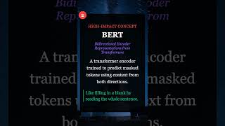
Comments Discord References
Concept Reference Regularization Dropout: A Simple Way to Prevent Neural Networks from Overfitting (Srivastava et al. 2014) BERT BERT: Pre-training of Deep Bidirectional Transformers (Devlin et al. 2018) RoPE RoFormer: Enhanced Transformer with Rotary Position Embedding (Su et al. 2021) Prompting Language Models are Few-Shot Learners (Brown et al. 2020) Positional Encoding Attention Is All You Need (Vaswani et al. 2017) Today’s Five
1. Regularization
Techniques that reduce overfitting by adding constraints or penalties during training. Common examples include L2 weight decay, L1 sparsity, dropout, and early stopping.
The goal is better generalization, not just fitting the training set.
Like adding friction so a model can’t take the easiest overfit path.
2. BERT
Bidirectional Encoder Representations from Transformers. A transformer encoder trained with masked language modeling: predicting hidden tokens using context from both sides.
It was a major step forward for many NLP tasks after its 2018 release.
Like filling in blanks by reading the whole sentence, not just the words before it.
3. RoPE (Rotary Positional Embeddings)
A way to represent token position inside attention by rotating query and key vectors as a function of position. This gives attention information about relative order and distance.
It’s widely used in modern transformer models.
Like turning a dial differently for each position so the model can tell where tokens are.
4. Prompting
Crafting inputs to steer a model toward the output you want. Small changes in instructions, examples, or format can change behavior significantly.
A key skill for working effectively with language models.
Like asking a question in just the right way to get a useful answer.
5. Positional Encoding
Transformers need a way to represent token order, because attention alone doesn’t include sequence position. Different methods do this, including learned embeddings and rotary approaches like RoPE.
Without it, “the cat sat on the mat” would be indistinguishable from “mat the on sat cat the.”
Like numbering the pages of a shuffled book so you can read them in order.
Quick Reference
Concept One-liner Regularization Add constraints to prevent overfitting BERT Bidirectional masked language modeling RoPE Position info via rotation in attention Prompting Craft inputs to steer model outputs Positional Encoding Tell the model where tokens are in sequence
Short, accurate ML explainers. Follow for more.
Part 6 of the Five ML Concepts series. View all parts | Next: Part 7 →
Comments or questions? SW Lab Discord or YouTube @SoftwareWrighter.
-
498 words • 3 min read • Abstract
Five ML Concepts - #5

5 machine learning concepts. Under 30 seconds each.
Resource Link Papers Links in References section Video Five ML Concepts #5 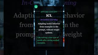
Comments Discord References
Concept Reference Perceptron The Perceptron: A Probabilistic Model (Rosenblatt 1958) Pre-training BERT: Pre-training of Deep Bidirectional Transformers (Devlin et al. 2018) Speculative Decoding Fast Inference from Transformers via Speculative Decoding (Leviathan et al. 2022) ICL Language Models are Few-Shot Learners (Brown et al. 2020) Latent Space Auto-Encoding Variational Bayes (Kingma & Welling 2013) Today’s Five
1. Perceptron
The simplest neural network: a single linear unit with weights and a bias. It computes a weighted sum and applies a threshold or activation.
It inspired modern neural networks, even though today’s models are far more complex.
Like a single voter weighing inputs before deciding yes or no.
2. Pre-training
Training a model on a large, general dataset before adapting it to a specific task. This gives the model broad patterns that later training can refine.
BERT, GPT, and most modern LLMs use this approach.
Like going to medical school before choosing a specialty.
3. Speculative Decoding
A technique where a small, fast model proposes tokens, and a larger model verifies or rejects them in parallel. This can speed up inference without changing final outputs.
A key optimization for production LLM deployments.
Like a junior writer drafting text for a senior editor to approve in batches.
4. In-Context Learning (ICL)
When a model adapts its behavior using examples in the prompt, without updating its weights. It allows flexible task behavior at inference time.
This emergent capability surprised researchers when GPT-3 demonstrated it.
Like solving a new puzzle after seeing a few worked examples.
5. Latent Space
The internal representations a model learns as it processes data. In this space, similar inputs tend to be located near each other.
It’s not a literal place, but a useful way to think about how models organize information.
Like a map where cities are arranged by similarity instead of geography.
Quick Reference
Concept One-liner Perceptron Single linear unit—the neural network ancestor Pre-training Learn general patterns before specializing Speculative Decoding Draft fast, verify in parallel ICL Adapt from prompt examples without training Latent Space Internal representations where similar things cluster
Related Posts
- In-Context Learning Revisited: From Mystery to Engineering — A deeper exploration of how ICL evolved from emergent surprise to engineered capability.
Short, accurate ML explainers. Follow for more.
Part 5 of the Five ML Concepts series. View all parts | Next: Part 6 →
Comments or questions? SW Lab Discord or YouTube @SoftwareWrighter.
-
458 words • 3 min read • Abstract
Five ML Concepts - #4

5 machine learning concepts. Under 30 seconds each.
Resource Link Papers Links in References section Video Five ML Concepts #4 
Comments Discord References
Concept Reference Activation Functions Deep Learning (Goodfellow et al. 2016), Chapter 6 Transfer Learning A Survey on Transfer Learning (Pan & Yang 2010) VLM Learning Transferable Visual Models (CLIP) (Radford et al. 2021) Adam Adam: A Method for Stochastic Optimization (Kingma & Ba 2014) Superposition Toy Models of Superposition (Elhage et al. 2022) Today’s Five
1. Activation Functions
Functions like ReLU, sigmoid, and tanh that transform neuron outputs. They introduce nonlinearity, allowing networks to learn complex patterns beyond simple linear relationships.
Without them, stacking layers would just be matrix multiplication.
Like an on-off switch that can also dim the lights.
2. Transfer Learning
Using knowledge a model learned on one task to improve performance on a related task. This often reduces training time and data requirements dramatically.
Pre-trained models can be fine-tuned for specific applications.
Like a chef who already knows French cooking learning Japanese cuisine faster.
3. VLM (Vision-Language Models)
Models trained to work with both images and text. They learn shared representations that connect visual and language understanding.
CLIP, GPT-4V, and LLaVA are examples of this approach.
Like someone who can look at a photo and describe what’s happening.
4. Adam
An optimizer that adapts learning rates for each parameter using information from past gradients. It combines ideas from momentum and adaptive learning-rate methods.
One of the most popular optimizers in deep learning.
Like a hiker who adjusts step size for each part of the trail, steep or flat.
5. Superposition
A way neural networks represent many concepts using overlapping directions in the same space. This allows models to pack more information into fewer neurons than expected.
It’s why interpretability is hard—features aren’t neatly separated.
Like discovering a painting has hidden layers that appear under the right light.
Quick Reference
Concept One-liner Activation Functions Introduce nonlinearity to enable complex patterns Transfer Learning Reuse knowledge from one task for another VLM Joint understanding of images and text Adam Adaptive per-parameter learning rates Superposition Many concepts packed into overlapping representations
Short, accurate ML explainers. Follow for more.
Part 4 of the Five ML Concepts series. View all parts | Next: Part 5 →
Comments or questions? SW Lab Discord or YouTube @SoftwareWrighter.
-
529 words • 3 min read • Abstract
Five ML Concepts - #3

5 machine learning concepts. Under 30 seconds each.
Resource Link Papers Links in References section Video Five ML Concepts #3 
Comments Discord References
Concept Reference Loss Function A Survey of Loss Functions for Deep Neural Networks (Janocha & Czarnecki 2017) Overfitting Dropout: A Simple Way to Prevent Neural Networks from Overfitting (Srivastava et al. 2014) Fine-tuning A Survey on Transfer Learning (Zhuang et al. 2020) LoRA LoRA: Low-Rank Adaptation of Large Language Models (Hu et al. 2021) Tokenization Neural Machine Translation of Rare Words with Subword Units (Sennrich et al. 2015) Today’s Five
1. Loss Function
A formula that measures how far off the model’s predictions are from the correct answers. It quantifies the gap between what the model predicted and what it should have predicted.
Training a neural network means minimizing this function.
Like a scorecard that tells the model how badly it messed up.
2. Overfitting
When a model learns the training data too well, including noise and outliers, and fails on new data. The model performs great on examples it has seen but poorly on anything new.
One of the most common pitfalls in machine learning.
Like memorizing the answers to a test instead of understanding the subject.
3. Fine-tuning
Taking a pre-trained model and training it further on a specific task or dataset. Instead of training from scratch, you start from a model that already understands language or images, then specialize it.
This makes powerful models accessible without massive compute budgets.
Like teaching a chef who already knows cooking to specialize in sushi.
4. LoRA (Low-Rank Adaptation)
An efficient fine-tuning method that trains a small number of added parameters instead of the full model. It inserts small trainable matrices into each layer while keeping the original weights frozen.
This dramatically reduces the memory and compute needed for fine-tuning.
Like adding sticky notes to a textbook instead of rewriting the whole thing.
5. Tokenization
The process of breaking text into smaller units called tokens that a model can process. Most modern models use subword tokenization, splitting words into common pieces rather than individual characters or whole words.
It determines what the model actually “sees” and affects everything from vocabulary size to multilingual performance.
Like chopping sentences into bite-sized pieces a model can digest.
Quick Reference
Concept One-liner Loss Function How far off the model’s predictions are Overfitting Memorizing the test instead of learning the subject Fine-tuning Specializing a pre-trained model for a new task LoRA Efficient fine-tuning with small added matrices Tokenization Breaking text into the pieces a model actually reads
Short, accurate ML explainers. Follow for more.
Part 3 of the Five ML Concepts series. View all parts | Next: Part 4 →
Comments or questions? SW Lab Discord or YouTube @SoftwareWrighter.
-
1784 words • 9 min read • Abstract
TBT #2: Pipelines on OS/390
Unix invented pipes. Mainframes reinvented them—for records, not bytes.
This is the second Throwback Thursday post—revisiting technologies that shaped how I think about programming. This time: CMS/TSO Pipelines, and a vibe coding project that brings them back to life in Rust for education, fun, and nostalgic reasons.
Resource Link Code pipelines-rs Demo Live Demo Video Pipelines on OS/390 #TBT Comments Discord The 1996 Olympics and a Pair of Mainframes
In 1996, IBM hosted the Olympics Web Server—one of the largest public web properties at the time. Many distributed IBM systems in different regions served dynamic web pages. The logs from all of them were funneled to a pair of IBM S/390 mainframes I was in charge of, running OS/390 (formerly MVS).
When you’re processing millions of log records for statistics and forensics, you need tools that think in records, not lines. That’s where Pipelines for TSO/E came in.
Pipelines for TSO/E was the MVS/ESA port of CMS Pipelines, which ran on VM/ESA. Both let you chain stages together to filter, transform, and aggregate record-oriented data—record-oriented pipelines that evolved in parallel with Unix’s byte-stream pipes.
Two Traditions of Piping
Unix pipes came first—Thompson and McIlroy at Bell Labs, 1969–1974. Byte streams, file descriptors, the
|operator. Brutally simple. Explosively powerful. POSIX.1-1988 standardizedpipe(2)and shell pipelines, though POSIX work began in the mid-1980s.CMS Pipelines emerged on IBM mainframes in the mid-to-late 1980s. They weren’t a Unix clone—they were convergent evolution under different pressures. Where Unix piped bytes between small programs, CMS piped records through declarative stages. Pipelines for TSO/E followed in the late 1980s and early 1990s, porting CMS concepts to the MVS multi-user environment. Unlike CMS Pipelines (which ships with z/VM), the TSO/E port is typically installed separately on z/OS.
Neither tradition was “behind.” They were optimizing different dimensions:
Unix Pipes CMS/TSO Pipelines Era 1969–1974 Mid-to-late 1980s Data unit Byte stream Records (fixed or variable length) Stage input stdin (bytes) Record buffer Field access awk,cut(text parsing)Column positions (direct) Execution Typically a process per stage Stages in one address space Topology Linear by default; fan-out/fan-in via tee, FIFOs, or process substitutionMulti-stream, fan-out/fan-in built in Philosophy Small tools, ad hoc composition Declarative data transformation Many datasets on mainframes are record-structured. Records can be fixed-length or variable-length. CMS and TSO/E Pipelines treat records as byte arrays—character-oriented stages assume EBCDIC text, while position/length stages are binary-safe. A fixed-length 80-byte record isn’t arbitrary text—columns 1-8 are the name, 9-18 are the department, 19-26 are the salary. You don’t parse. You just read the right columns.
Unix won culturally—cheap hardware, academic distribution, C portability. But IBM’s record-oriented pipelines were better at structured dataflow, and they anticipate or parallel patterns seen in ETL frameworks like Spark and Beam.
CMS Pipelines ships with z/VM and is still used; Pipelines for TSO/E exists for z/OS but isn’t universally installed. These are not historical curiosities—mainframes continue to process a significant share of high-value transactions, and pipelines remain an available tool for data transformation on those systems.
What a Pipeline Looks Like
CMS Pipelines uses a DSL with
PIPEas the command,|to chain stages, and?as a command terminator (it suppresses the console from being used as implicit input):PIPE CONSOLE | FILTER 18,10 = "SALES" | SELECT 0,8,0; 8,10,8 | CONSOLE ?This reads input records, keeps only those where columns 18–27 equal “SALES”, extracts the name fields, and writes the result. No regex. No string splitting. Just column positions.
Note: pipelines-rs uses 0-based offsets (e.g.,
SELECT 0,8,0). Historical CMS Pipelines uses 1-based column positions.Compare with the Unix equivalent:
cat input.txt | awk '$3 == "SALES" {print $1, $2}'The Unix version looks simpler—until your fields contain spaces, or your records contain non-text bytes, or you need to chain 15 stages without spawning 15 processes.
Bringing It Back in Rust (Vibe Coding)
pipelines-rs is a nostalgia-driven vibe coding project—my attempt to emulate Pipelines for TSO/E in Rust, not because it’s practical, but because these ideas deserve to be celebrated. It supports a subset of stages and features two execution models:
The Two Executors
Batched processes all records through one stage before moving to the next:
All records → Stage 1 → All records → Stage 2 → All records → Stage 3This emulates the correct output and is faster, but doesn’t demonstrate record-oriented dataflow well.
Record-At-a-Time (RAT) sends each record through the entire pipeline before reading the next:
Record 1 → Stage 1 → Stage 2 → Stage 3 → Output
Record 2 → Stage 1 → Stage 2 → Stage 3 → Output
Record 3 → Stage 1 → Stage 2 → Stage 3 → Output
RAT is the implementation shown in the video. It’s a naive approach—more buffers, more copying—but it shows the dataflow concepts clearly and enables the visual debugger. Both run in linear time (records × stages) and produce identical output for all 23 test specifications.
A future version will aim for fewer buffers and fewer copy operations. Whether it’s faster than Batched remains to be seen.
The 80-Byte Record
The Rust implementation supports fixed-length records only. The fundamental data type is the
Record—exactly 80 bytes, matching historical punch card width. Variable-length input lines are accepted and padded to 80 bytes:pub const RECORD_WIDTH: usize = 80; pub struct Record { data: [u8; RECORD_WIDTH], }Fields are accessed by column position and length. No parsing, no delimiters. The data is always right where you expect it.
Supported Stages
The current implementation supports 14 stages:
Stage Purpose Example FILTER Keep/reject records by field value FILTER 18,10 = "SALES"LOCATE Keep records containing a pattern LOCATE "ERROR"NLOCATE Keep records NOT containing a pattern NLOCATE "DEBUG"SELECT Extract and reposition fields SELECT 0,8,0; 8,10,8CHANGE Text replacement CHANGE "SALES" "MKTG"COUNT Count records COUNTTAKE Keep first N records TAKE 5SKIP Skip first N records SKIP 2DUPLICATE Repeat each record N times DUPLICATE 3LITERAL Append a literal record LITERAL "--- END ---"UPPER/LOWER Case conversion UPPERREVERSE Reverse record text REVERSEHOLE Discard all input HOLECONSOLE Driver stage: source or sink depending on position CONSOLEThe CLI
Both executors have identical CLIs:
# Batch executor
pipe-run specs/filter-sales.pipe specs/input-fixed-80.data -v

# Record-at-a-time executor
pipe-run-rat specs/filter-sales.pipe specs/input-fixed-80.data -v
Given this input data:
SMITH   JOHN      SALES     00050000
JONES   MARY      ENGINEER  00075000
DOE     JANE      SALES     00060000
WILSON  ROBERT    MARKETING 00055000
CHEN    LISA      ENGINEER  00080000
GARCIA  CARLOS    SALES     00045000
TAYLOR  SUSAN     MARKETING 00065000
BROWN   MICHAEL   ENGINEER  00090000
And this pipeline:
PIPE CONSOLE
| FILTER 18,10 = "SALES"
| CONSOLE
?
The output is:
SMITH   JOHN      SALES     00050000
DOE     JANE      SALES     00060000
GARCIA  CARLOS    SALES     00045000
Records:  8 in -> 3 out
Exactly what I’d have gotten on OS/390 in 1996, but with Web Server log data showing client IP address, OS, browser type/version, user cookies, timestamps, URLs, and more, instead of accounting data. 😊
The Web UI for Two pipelines-rs Implementations
The web interface runs entirely in the browser via WebAssembly. It has three panels: input records with an 80-column ruler, the pipeline editor, and the output.
Tutorial Mode
The tutorial walks through each stage with examples, running pipelines automatically to show results. You can step through manually or let it auto-advance.
The Visual Debugger
The debugger is the reason RAT exists. It lets you:
- Step through execution one pipe point at a time
- Watch data at specific pipe points between stages
- Set breakpoints to pause at specific stages
- See stage state for stateful stages like COUNT
You load a pipeline, click Run, then Step to watch each record flow through each stage. The debugger highlights which stages have been reached with a green border. For COUNT and other aggregation stages, you can watch the flush phase where accumulated state becomes output.
What’s Next
The current RAT executor is intentionally naive—it uses a buffer at every pipe point and copies each record between them. A better implementation would minimize buffers and copy operations while preserving the record-at-a-time semantics.
Multi-pipe features are also planned—CMS Pipelines supported fan-out (one input, multiple output streams) and fan-in (multiple inputs merged), which enabled complex processing topologies beyond simple linear chains.
How pipelines-rs Differs from IBM Pipelines
IBM CMS/TSO/E Pipelines pipelines-rs Indexing 1-based column positions 0-based offsets Record format Fixed or variable length, EBCDIC Fixed 80-byte ASCII only (variable-length input padded) Stages Hundreds of built-in stages 14 implemented so far Topology Multi-stream: fan-out, fan-in, multi-pipe Linear only (multi-pipe planned) Environment z/VM, z/OS mainframes CLI (native) and browser (WASM) Character set EBCDIC ASCII/UTF-8 This is a teaching tool and nostalgia project, not a production replacement.
Implementation Details
Metric Value Language Rust (2024 edition) Web UI Yew framework, compiled to WASM Stages 14 implemented Test Specs 23 pipeline specifications Tests 60+ (including batch/RAT equivalence) License MIT Live Demo sw-comp-history.github.io/pipelines-rs Resources
Credits
Role Who Concept & direction Mike Wright Content creation Claude (Anthropic) Editorial review ChatGPT (OpenAI)
Mainframe ideas, modern tools. Follow for more.
Part 2 of the Throwback Thursday series. View all parts | Next: Part 3 →
Comments or questions? SW Lab Discord or YouTube @SoftwareWrighter.
-
979 words • 5 min read • Abstract
Small Models (6/6): Which Small AI Fits YOUR Laptop?

Maximum AI capability on minimum hardware. The 2-3B efficient frontier.
This is Part 6 (the finale) of the Small Models, Big Brains series. We’re benchmarking the best small models to help you choose the right one for your laptop.
Resource Link Code efficient-llm Phi-2 microsoft/phi-2 Gemma ai.google.dev/gemma SmolLM HuggingFace Blog Video Which Small AI Fits YOUR Laptop? 
Comments Discord The Efficient Frontier
In economics, the “efficient frontier” is the set of optimal portfolios offering the highest return for a given level of risk.
In AI, it’s the models offering the best capability for a given size.
The Contenders
Model Params Source Key Strength Phi-2 2.7B Microsoft Reasoning, synthetic data Gemma-2B 2B Google Distillation, multilingual SmolLM2-1.7B 1.7B HuggingFace 11T tokens, fast inference SmolLM3-3B 3B HuggingFace Dual reasoning, 6 languages Benchmark Results
Actual measurements on Apple Silicon (M-series) from efficient-llm:
Model MMLU GSM8K HumanEval Speed (CPU) Memory Phi-2 61.7% 57.0% 50.0% 7.1 tok/s 5.2GB Gemma-2B 38.9% 18.0% 90.0% 8.5 tok/s 4.7GB SmolLM2 55.6% * * 3.7 tok/s 3.2GB *SmolLM2 GSM8K/HumanEval scores reflect prompt format incompatibility, not capability.
The Key Insight: Data Quality Beats Parameters
Phi-2 achieves 61.7% MMLU with only 2.7B parameters.
For comparison:
- Llama-2-7B: ~46% MMLU
- Llama-2-13B: ~55% MMLU
Phi-2 beats models 5x its size. The secret? Synthetic textbook training.
Microsoft generated high-quality educational content specifically designed to teach reasoning. Quality data > quantity data > model size.
Model Profiles
Phi-2: The Reasoning Champion
Strengths: Math, logic, code understanding
Weakness:  Less conversational
Best for:  Technical tasks, chain-of-thought
Phi-2 was trained on “textbook quality” synthetic data. It thinks like a textbook explains.
Gemma-2B: The Distillation Expert
Strengths: Multilingual, edge deployment
Weakness:  Lower benchmark scores
Best for:  Production apps, Google ecosystem
Google distilled knowledge from larger models into this compact package. Great tooling and documentation.
SmolLM2-1.7B: The Speed Demon
Strengths: Fastest inference, smallest footprint
Weakness:  Prompt format sensitivity
Best for:  Memory-constrained environments
HuggingFace trained on 11T tokens—massive overtraining like TinyLlama but at a slightly larger scale.
SmolLM3-3B: The Balanced Choice
Strengths: Dual reasoning modes, 6 languages
Weakness:  Newest, less battle-tested
Best for:  General-purpose small model needs
The latest from HuggingFace, designed to be the go-to small model.
Decision Framework
├── Need best reasoning?           → Phi-2
├── Need instruction following?    → SmolLM2 or SmolLM3
├── Need multilingual?             → Gemma-2B or SmolLM3
├── Memory constrained (<4GB)?     → SmolLM2 + INT4
├── Need Google ecosystem?         → Gemma-2B
├── General purpose?               → SmolLM3
└── Maximum quality per byte?      → Phi-2
Running the Benchmarks
git clone https://github.com/softwarewrighter/efficient-llm
cd efficient-llm

# Setup
uv venv && source .venv/bin/activate
uv pip install torch transformers accelerate bitsandbytes datasets tqdm

# HuggingFace login (required for Gemma)
huggingface-cli login

# Download and benchmark
python download_models.py
python benchmark_quality.py
python benchmark_speed.py
python benchmark_memory.py

# Interactive demos
python demo_reasoning.py
python demo_code.py
python demo_chat.py
Hardware Requirements
Setup Models You Can Run 4GB RAM SmolLM2 (INT4) 8GB RAM All models (INT4) 16GB RAM All models (FP16) Apple Silicon All models (MPS) Implementation Details
Metric Value Primary Language Python Source Files 7 .pyfilesEstimated Size ~1.4 KLOC Framework Transformers, PyTorch Build System uv / pip Key Features MMLU/GSM8K/HumanEval benchmarks, demos Good for you if: You want to benchmark 2-3B models, compare quality vs speed tradeoffs, or run interactive comparisons between Phi-2, Gemma, and SmolLM.
Complexity: Low. Similar structure to billion-llm. Standalone Python scripts for each benchmark and demo. Requires HuggingFace authentication for Gemma access.
Series Recap
Over six parts, we’ve explored the cutting edge of small model research:
Part Model/Topic Key Insight 1 TRM (<1K params) Iteration beats scale 2 MobileLLM (350M) Offline AI is practical 3 HRM (27M) Hierarchy enables reasoning 4 BDH Sparsity enables interpretability 5 1B models The efficiency sweet spot 6 2-3B models Data quality beats parameters Key Takeaways
-
Data quality beats parameter count. Phi-2 proves careful curation outperforms brute scaling.
-
The 2-3B range is remarkably capable. These models handle real tasks, not just demos.
-
Each model has its niche. Match the model to your use case.
-
Quantization makes everything accessible. INT4 lets you run 3B models on 4GB RAM.
-
The frontier keeps moving. SmolLM3 is weeks old. Better models are coming.
What We’ve Learned
Small models aren’t a compromise—they’re a different optimization target. When you can’t throw compute at a problem, you’re forced to be clever:
- Recursive reasoning (TRM)
- Mobile-optimized architectures (MobileLLM)
- Hierarchical decomposition (HRM)
- Sparse interpretable activations (BDH)
- Overtraining on quality data (TinyLlama, Phi-2)
These techniques will eventually feed back into large models too. Small model research isn’t a dead end—it’s the frontier.
Resources
Part 6 of 6 in the Small Models, Big Brains series. Thanks for following along!
Part 6 of the Small Models, Big Brains series. View all parts
Comments or questions? SW Lab Discord or YouTube @SoftwareWrighter.
-
451 words • 3 min read • Abstract
Five ML Concepts - #2

5 machine learning concepts. Under 30 seconds each.
Resource Link Papers Links in References section Video Five ML Concepts #2 
Comments Discord References
Concept Reference Gradient Descent An overview of gradient descent optimization algorithms (Ruder 2016) Attention Neural Machine Translation by Jointly Learning to Align and Translate (Bahdanau et al. 2014) DPO Direct Preference Optimization (Rafailov et al. 2023) Learning Rate Cyclical Learning Rates (Smith 2015) Temperature On the Properties of Neural Machine Translation (Cho et al. 2014) Today’s Five
1. Gradient Descent
A general optimization method used across machine learning. It improves a model by taking small steps in the direction that reduces error the most.
Many learning algorithms rely on it, especially neural networks.
Like walking downhill in fog, adjusting each step based on the slope beneath your feet.
2. Attention
A mechanism that lets models weigh different parts of the input by importance. Instead of treating everything equally, attention highlights what matters most.
This was key to breakthroughs in translation and language models.
Like reading a sentence and focusing more on the important words.
3. DPO (Direct Preference Optimization)
A method for aligning language models with human preferences. Unlike RLHF, it trains directly on preference comparisons and avoids an explicit reward model.
This simplifies training while achieving comparable alignment.
Like learning preferences by observing choices, not by designing a scoring system.
4. Learning Rate
Controls how large each update step is during training. Too large and learning becomes unstable. Too small and training is slow or gets stuck.
One of the most important hyperparameters to tune.
Like choosing how fast to walk downhill without losing balance.
5. Temperature
A parameter that controls randomness during text generation. Low temperature favors predictable, high-probability outputs. Higher temperature increases variety and surprise.
A tradeoff between consistency and creativity.
Like adjusting a dial from cautious to adventurous.
Quick Reference
Concept One-liner Gradient Descent Walk downhill to minimize error Attention Focus on what matters in the input DPO Align models from preference pairs directly Learning Rate Step size that balances speed and stability Temperature Dial between predictable and creative
Short, accurate ML explainers. Follow for more.
Part 2 of the Five ML Concepts series. View all parts | Next: Part 3 →
Comments or questions? SW Lab Discord or YouTube @SoftwareWrighter.
-
844 words • 5 min read • Abstract
Small Models (5/6): Max AI Per Watt

One billion parameters. The sweet spot for AI.
Big enough to reason. Small enough to run anywhere. Maximum capability per watt.
This is Part 5 of the Small Models, Big Brains series, comparing four models at the 1B parameter point.
Resource Link Code billion-llm TinyLlama jzhang38/TinyLlama Llama 3.2 ai.meta.com/llama Pythia EleutherAI/pythia Video Max AI Per Watt 
Comments Discord Why One Billion?
Range Reality Below 1B Models struggle with complex reasoning Above 1B Hardware requirements increase significantly At 1B Maximum capability per watt 1B parameters is where you get:
- Real language understanding
- Ability to follow instructions
- Fine-tuning in minutes on a laptop
- Deployment anywhere (phone, Raspberry Pi, browser)
The Contenders
Model Params Key Strength Training Data TinyLlama 1.1B Overtrained on 3T tokens Community Llama-3.2-1B 1B Official Meta ecosystem Meta StableLM-1.6B 1.6B Multilingual, 2T tokens Stability AI Pythia-1B 1.08B 154 research checkpoints EleutherAI TinyLlama: The Overtraining Champion
TinyLlama breaks the rules. The Chinchilla scaling laws suggest training tokens should scale with parameters. TinyLlama uses 100x more data than optimal.
Chinchilla-optimal for 1B: ~30B tokens
TinyLlama actual:          3T tokens (3,000B)
The result? A tiny model that punches well above its weight.
Benchmarks
From the billion-llm repository:
Model MMLU HumanEval Speed Memory TinyLlama 25.3% 12.2% Fast 2.2GB Llama-3.2-1B 32.1% 18.5% Fast 2.4GB StableLM-1.6B 30.8% 15.1% Medium 3.2GB Pythia-1B 26.4% 10.3% Fast 2.2GB Llama-3.2-1B leads on quality. TinyLlama offers the best value when you factor in the open training recipe.
LoRA Fine-Tuning in Minutes
All these models can be fine-tuned on a laptop using LoRA:
cd billion-llm
python finetune_demo.py --model tinyllama --epochs 3
LoRA adds small trainable adapters without modifying base weights:
Base Model (frozen): 1.1B parameters
LoRA Adapters:       ~4M parameters (0.4%)
Training time:       5-10 minutes on M1 Mac
Speculative Decoding: 2-3x Speedup
Use a fast 1B model to draft tokens, verify with a slower 7B model:
Draft (1B):   "The quick brown fox" → [jumps, over, the, lazy]
Verify (7B):  Accept [jumps, over, the] → Reject [lazy] → Generate [sleepy]
The 1B model generates candidates quickly. The 7B model only needs to verify, not generate from scratch.
python speculative_demo.pyResults: 2-3x speedup on autoregressive generation.
Hardware Requirements
Setup What You Can Run CPU only All models (slower, INT4 quantized) 4GB VRAM All models (INT4 quantized) 8GB VRAM All models (FP16) Apple Silicon All models (MPS acceleration) Quick Start
git clone https://github.com/softwarewrighter/billion-llm
cd billion-llm

# Setup
uv venv && source .venv/bin/activate
uv pip install -r requirements.txt

# Download models
python download_models.py

# Run benchmarks
python benchmark.py

# Interactive comparison
python demo_chat.py --compare tinyllama llama3.2-1b
Which Model Should You Choose?
├── Need Meta ecosystem compatibility? → Llama-3.2-1B
├── Need multilingual support?         → StableLM-1.6B
├── Need research reproducibility?     → Pythia-1B (154 checkpoints)
├── Need maximum performance/size?     → TinyLlama
└── Just getting started?              → Any of them work!
Implementation Details
Metric Value Primary Language Python Source Files 8 .pyfilesEstimated Size ~1.4 KLOC Framework Transformers, PyTorch Build System uv / pip Key Features Benchmarking, LoRA fine-tuning, speculative decoding Good for you if: You want to benchmark small LLMs, learn LoRA fine-tuning, experiment with speculative decoding, or compare models head-to-head.
Complexity: Low. Clean Python scripts with HuggingFace Transformers. Each script is standalone—run benchmarks, chat demos, or fine-tuning independently. Well-documented with shell scripts for common tasks.
Key Takeaways
-
1B is the efficiency sweet spot. Below this, capability drops. Above, hardware costs rise.
-
Overtraining works. TinyLlama proves you can compensate for size with data.
-
LoRA makes fine-tuning accessible. Customize models on consumer hardware.
-
Speculative decoding is free speed. Use small models to accelerate large ones.
-
All roads lead to open weights. Every model here is fully open.
What’s Next
Part 6 explores the 2-3B efficient frontier—Phi-2, Gemma, and SmolLM pushing the limits of small model capability.
Resources
- billion-llm Repository
- TinyLlama
- Llama 3.2
- Pythia
- LoRA Paper
- Speculative Decoding Paper
- Video: Max AI Per Watt
Part 5 of the Small Models, Big Brains series. View all parts | Next: Part 6 →
Comments or questions? SW Lab Discord or YouTube @SoftwareWrighter.
subscribe via RSS